PPOL 6801 - Text as Data - Computational Linguistics


Week 6: Unsupervised Learning:
Topic Models

Professor: Tiago Ventura

Housekeeping

Let’s quickly review your future assignments:

  • Problem Set 1

    • Read instructions: Submit your qmd compiled.
    • Issues with GitHub: update your PAT. You probably do not have permission to post on a org repo.
    • Grades to be posted soon (just have a few more to go through)
  • Problem Set 2

    • Coming soon ~ In two weeks, no class next week.
  • Project Proposal

    • EOD Friday Week 8 ~ Oct 31
      • you have to meet with me before submitting your proposal
      • Send me a draft of the proposal before the meeting

Coding: Supervised Learning

Where are we?

We started from pre-processing text as data, representing text as numbers, describing features of the tex, and learned how to measure concepts in text:

  • Last Week: Supervised learning ~ Training your models
    • Crowdsourcing label classification
    • Full pipeline for model training
    • Regularized regressions
    • Evaluating Performance
  • This week: unsupervised learning

Overview: Unsupervised Learning

  • Data: humans, documents, votes, etc. are not pre-labelled in terms of some underlying concept.

    • Think about congressional speeches, we know the author, their party, other metadata, but:
      • We don’t yet know what that speech ‘represents’ in terms of its latent properties, what ‘kind’ of speech it is, what ‘topics’ it covers, what speeches it is similar to conceptually, etc.
  • Goal: take the observations and find hidden structure and meaning in them

    • similarity
    • groups
    • topics
    • association between word, etc…
  • Main models we will learn:

    • Clustering Models

    • Topic Models

Main challenges of Unsupervised Learning

Hard to get it right

  • Unsupervised learning requires several ad-hoc decisions and these decisions matter for quality of your results

    • number of clusters
    • number of topics
    • pre-processing steps
  • Domain knowledge (and honestly a bit of randomness) guides a lot of these decisions

Hard to know if you are doing right!

  • In contrast to supervised approaches, we won’t know ‘how correct’ the output

  • Use statistical measures of fit/unfit of different modeling decisions

    • but in general, it will involve a hugely amount of qualitative assessment.
  • No easy measure of accuracy, recall and precision.

Clustering Methods

Problem

Purpose: look for ‘groups’ in data explicitly.

  • Input: text + number of clusters
  • Output: documents ~> clusters

Clusters: group of data points that are all nearby to each other and far away from other clusters.

Research Questions? How can we categorize these news articles or policy bills? How can we group these legislators based on their speeches?

K-means clustering

K-Means clustering: partition the docs into a set of K categories where docs with similar rates of word usage are assigned to the same cluster and dissimilar docs are assigned to different categories

  1. Pre-specify cluster numbers

  2. Algorithm puts observations into clusters which minimize the within-cluster sum of squares (i.e., sum of squared Euclidean distances between each data point and its assigned cluster centroid)

  3. Objective function to minimize

K-Means Steps

  • Initialize Clusters centroids randomly (\(\mu_k\))

  • Assign Documents to nearest centroid clusters using euclidean distance.

  • Calculate loss function between points and their clusters

\[ J = \sum_{i=1}^{n} \sum_{k=1}^{K} r_{ik} \, \| x_i - \mu_k \|^2 \]

  • Update centroids

\[ \mu_k = \frac{\sum_{i=1}^{n} r_{ik} \, x_i}{\sum_{i=1}^{n} r_{ik}} \]

  • Repeat (from bullet point 2) until convergence.

Visually

Visually

Visually

Visually

Algorithm

Clustering vs Topic Models

Topics models can be thought as a probabilistic generalization of clustering methods

Algorithmic vs Probabilistic Models

Algorithmic Models Probabilistic Models
Idea learning as an optimization problem learning as inference based on mathematical model aboout the world
Output Deterministic representations (e.g., clusters, embeddings) Distributions + uncertainty over latent structures
Goal minimize a cost function Estimate the likelihood of observed data given certain parameters

Clustering vs Topic Models

  • Clustering:

    • Every document is assigned to a cluster that minimizes a cost function
  • Topic Models:

    • every document has a probability distribution of topic.

    • every topic has a probability distribution of words.

    • use likelihood estimation to find the parameters of these distributions

Topic Models: Intuition

  • Problem: Once we start with docs, we do not know what topics exist, what words belong to which topics, what topic proportions each document has

  • Probabilistic Model: Make assumptions about how language work, and how topics emerge:

  • Documents: formed from probability distribution of topics

    • a speech can be 40% about trade, 30% about sports, 10% about health, and 20% spread across topics you don’t think make much sense
  • Topics: formed from probability distribution over words

    • the topic health will have words like hospital, clinic, dr., sick, cancer

Latent Dirichlet Allocation: LDA

Intuition: Language Model

  • Step 1: For each document:

    • Randomly choose a distribution over topics. That is, choose one of many multinomial distributions, each which mixes the topics in different proportions.
  • Step 2: For each topic

    • Randomly choose a distribution of words, also from one of many multinomial distributions., each with mixes words in different proportions
  • Step 3: Then, for every word in the document

    • Randomly choose a topic from the distribution over topics from step 1.
    • Randomly choose a word from the distribution over the vocabulary that the topic implies.

Step 1 and 2: or what a multinomial distribution looks like

For each document (and then topic) ~ Randomly choose a distribution from many multinomal distributions

Step 2: sampling words

For every word:

  • Randomly choose a topic from the distribution over topics from step 1.

  • Randomly choose a word from the distribution over the vocabulary that the topic implies.

Latent Dirichlet Allocation

To estimate the model, we need to assume some known mathematical distributions for this data generating process:

  • For every topic: Each topic k has a word distribution \(\beta_k\) , drawn from a Dirichlet prior:

    • \(\beta_k \sim \text{Dirichlet}(\tau)\)
  • For every document: Each document d has a topic distribution \(\theta_d\) , drawn from a Dirichlet prior

    • \(\theta_d \sim \text{Dirichlet}(\alpha)\),
  • For every word:

    • For each word wdn in document d, choose a topic \(z_{dn}\) based on the document’s topic distribution, a topic \(z_{dn} \sim \text{Multinomial}(\theta_d)\).
    • Choose a word \(w_{dn}\) from the topic’s word distribution: \(w_{dn} \sim \text{Multinomial}(\beta_{z_{dn}})\)
  • where:

    • \(\alpha\) and \(\tau\) are hyperparameter of the Dirichlet priors
    • \(\beta_k\) is drawn from a Dirichlet for per-topic word distribution
    • \(\theta_d\) is drawn from a Dirichlet for the topic distribution for documents - \(K\) topics
    • \(D\) documents in the corpus
    • \(dn\) word position in document \(d\)

Aside: Dirichlet distribution

  • The Dirichlet distribution is a conjugate prior for the multinomial distribution.

    • It makes joint distributions easier to calculate because we know their families.
  • It is parameterized by a vector of positive real numbers (\(alpha\))

    • Larger values of \(\alpha\) (assuming we are in symmetric case) mean we think (a priori) that documents are generally an even mix of the topics.

    • If \(\alpha\) is small (less than 1) we think a given document is generally from one or a few topics.

Visually

Inference: How to estimate all these parameters?

Inference: Use the observed data, the words, to make an inference about the latent parameters: the \(\beta\)s, and the \(\theta\)s.

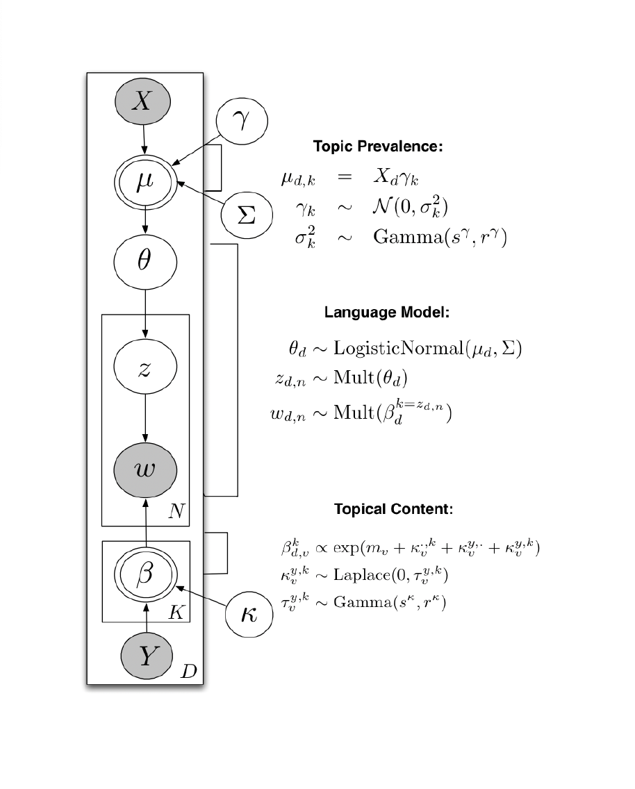
We start with the joint distribution implied by our language model (Blei, 2012):

\[ p(\beta_{1:K}, \theta_{1:D}, z_{1:D}, w_{1:D})= \prod_{K}^{i=1}p(\beta_i)\prod_{D}^{d=1}p(\theta_d)(\prod_{N}^{n=1}p(z_{d,n}|\theta_d)p(w_{d,n}|\beta_{1:K},z_{d,n}) \]

To get to the conditional:

\[ p(\beta_{1:K}, \theta_{1:D}, z_{1:D}|w_{1:D})=\frac{p(\beta_{1:K}, \theta_{1:D}, z_{1:D}, w_{1:D})}{p(w_{1:D})} \]

The denominator is hard complicate to be estimate (requires integration for every word for every topic):

  • Simulate with Gibbs Sampling or Variational Inference (Bayesian stats)

Show me results!

Choosing the number of topics

  • Choosing K is “one of the most difficult questions in unsupervised learning” (Grimmer and Stewart, 2013, p.19)

  • Common approach: decide based on cross-validated statistical measures model fit or other measures of topic quality.

Validation of topics

  • Working with topic models require a lot of back-and-forth and humans in the loop.

  • How to measure the quality of the topics?

  • Crowdsourcing for:

    • whether a topic has (human-identifiable) semantic coherence: word intrusion, asking subjects to identify a spurious word inserted into a topic
    • whether the association between a document and a topic makes sense: topic intrusion, asking subjects to identify a topic that was not associated with the document by the model
    • See Ying et al, 2022, Political Analysis.
  • Contextual Knowledge, reading the topics, and showing it has face-validity.

Applications

Barbera et al, American Political Science Review, 2020.

  • Data: tweets sent by US legislators, samples of the public, and media outlets.

  • LDA with K = 100 topics

  • Topic predictions are used to understand agenda-setting dynamics (who leads? who follows?)

  • Conclusion: Legislators are more likely to follow, than to lead, discussion of public issues,

Motolinia, American Political Science Review, 2021

  • Data: transcripts of legislative sessions in Mexican states
  • Correlated Topic model to identify “particularistic” legislation; i.e. laws with clear benefits to voters
  • Each topic is then classified into particularistic or not
  • Validation: correlation with spending
  • Use exogenous electoral reform that allowed legislators to be re-elected

Exercise

  • Take 5-min to read the methods sections of these papers

  • List to me some of the decisions the authors need to make to get the topic models to work.

  • Do you think these make sense? What would you do different?

Extensions: Many more beyond LDA

  • Structural topic model: allow (1) topic prevalence, (2) topic content to vary as a function of document-level covariates (e.g., how do topics vary over time or documents produced in 1990 talk about something differently than documents produced in 2020?); implemented in stm in R (Roberts, Stewart, Tingley, Benoit)

  • Correlated topic model: way to explore between-topic relationships (Blei and Lafferty, 2017); implemented in topicmodels in R; possibly somewhere in Python as well!

  • Keyword-assisted topic model: seed topic model with keywords to try to increase the face validity of topics to what you’re trying to measure; implemented in keyATM in R (Eshima, Imai, Sasaki, 2019)

  • BertTopic: BERTopic is a topic modeling technique that leverages transformers and TF-IDF to create dense clusters of words.

STM: Adding Structure to the LDA


  • Prevalence: Prior on the mixture over topics is now document-specific, and can be a function of covariates.

  • Content: distribution over words is now document-specific and can be a function of covariates.

See Roberts et al 2014

Quick survey: click here

Coding!