PPOL 6801 - Text as Data - Computational Linguistics
Week 8: Introduction to Deep Learning
Professor: Tiago Ventura
Plans for Today
Mid-semester survey
Overview of where we are going
Introduction to Deep Learning
Mid-Semester Survey:
Start doing
Recording a video going through the code we’re going over in class that day
Explaining more about the assignments
Move the coding exercise to the same day
Explain more about the code
While coding in class is helpful, I’d appreciate a slightly deeper dive into concepts.
maybe advice going through coding material before or after class. because doing it on the class is too time consuming
Stop Doing
going through the code in class
I don’t think we need to devote as much time to coding
Maybe just have us read the paper that will be covered in the upcoming class,
the morning-3-hour-class, lol
I personally don’t find the textbook very helpful
I would spend less time on the earlier methods that aren’t really used anymore
Continue Doing
I appreciate the readings a lot and I wish we had more time dedicated to talking through them. (LET ME KNOW WHICH! HELP TO DO THAT)
Everything is nice in PPOL 6801 (THANK YOU!)
Going over the R code in class! I like the half code, half lecture style.
Overall, I think the class is pretty well curated!
Most useful material
- Problem sets with 54%!
Where we are going…
We are living through a fast pacing transformation on the use of text-as-data
The most recent changes come from the so called Large Langue Models, and their increasing capability of generating human-like text.
This revolution was enabled by:
Increasing accessibility to data
Better ways to represent word
Use of deep learning architectures to model text.
Neural Networks - Transformers (2017)
For us to understand this figure, we should first:
Grasp the basic concepts of how a neural network model operates
Understand the idea of dense representation of words (word vectors) vs Sparse Representation (DFMs)
Understand attention mechanisms
Get to transformers
Our plans for the next few weeks
today: introduction to deep learning
next: word embeddings
next, next: applications of word embeddings
next, next, next: break for your replication
next, next, next,next: Transformers (attention is all you need)
next, next, next, next, next: LLMs
Text Representation: From Sparse to Dense Vectors
Vector Space Model
To represent documents as numbers, we learned about the vector space model representation:
A document \(D_i\) is represented as a collection of features \(W\) (words, tokens, n-grams..)
Each feature \(w_i\) can be place in a real line, then a document \(D_i\) is a point in a \(W\) dimensional space
Imagine the sentence below: “If that is a joke, I love it. If not, can’t wait to unpack that with you later.”
Sorted Vocabulary =(a, can’t, i, if, is, it, joke, later, love, not, that, to, unpack, wait, with, you”)
Feature Representation = (1, 1, 1, 2, 1, 1, 1, 1, 1, 1, 2, 1, 1, 1, 1, 1)
Features will typically be the n-gram (mostly unigram) frequencies of the tokens in the document, or some function of those frequencies
Now each document is now a vector (vector space model)
- stacking these vectors will give you our workhose representation for text: Document Feature Matrix
Documents
Document 1 = “yes yes yes no no no”
Document 2 = “yes yes yes yes yes yes” :::
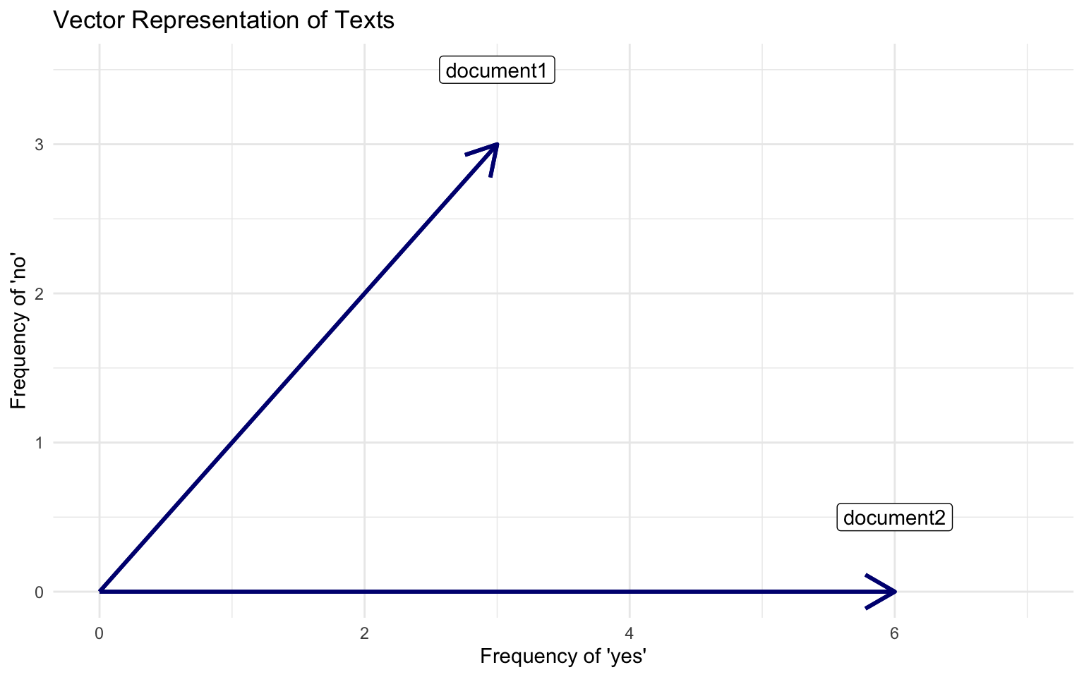
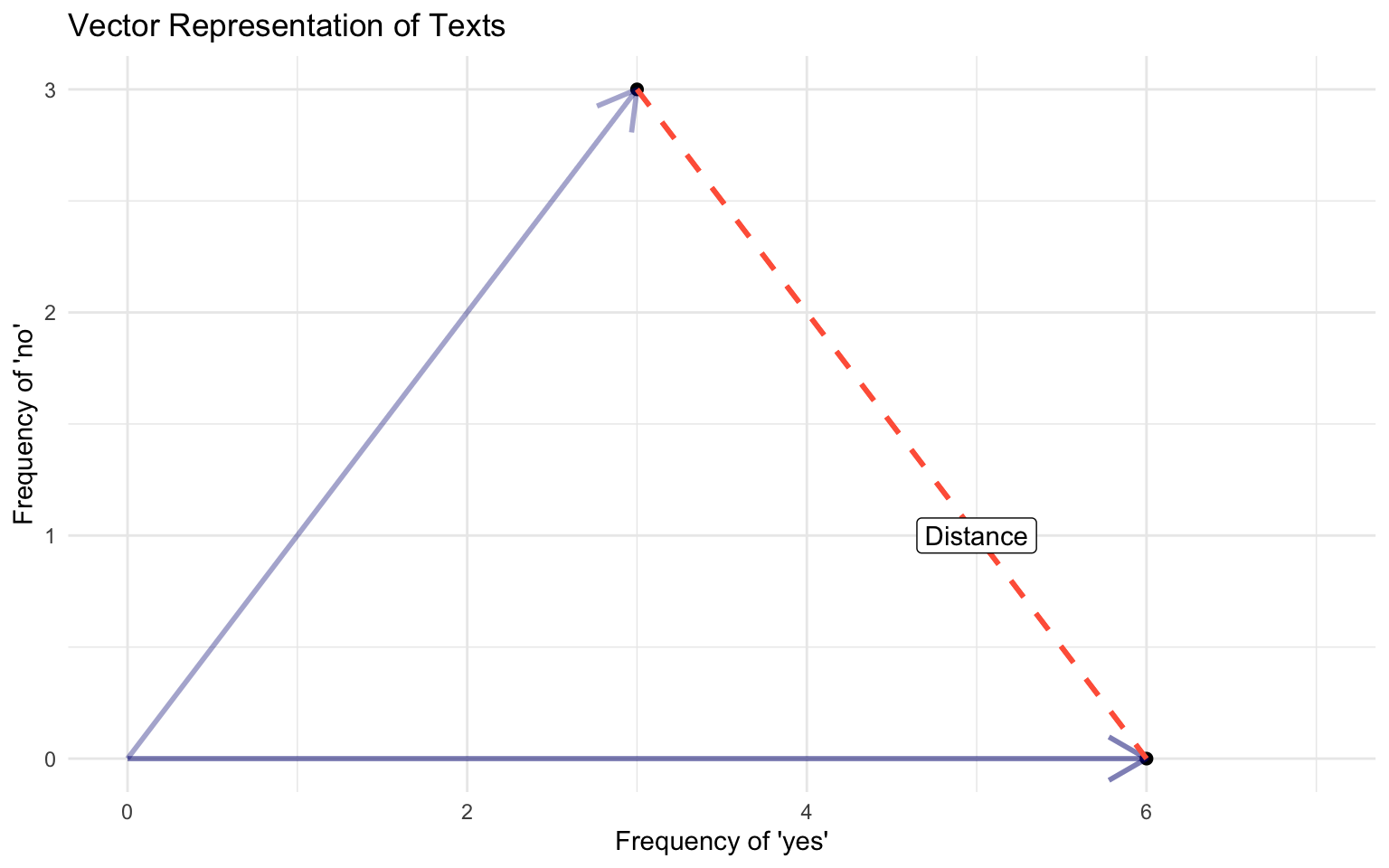
Visualizing Vector Space Model
In the vector space, we can use geometry to build well-defined comparison measures between the documents
Vector Space Model vs Representation Learning
The vector space model is super useful, and has been used in many many many applications in computational linguistics and social science applications of text-as-data. Including:
Descriptive statistics of documents (count words, text-similarity, complexity, etc..)
Supervised Machine Learning Models for Text Classification (DFM becomes the input of the models)
Unsupervised Machine Learning (Topic Models & Clustering)
But… Embedded in this model, there is the idea we represent words as a one-hot encoding.
- “cat”: [0,0, 0, 0, 0, 0, 1, 0, ….., V] , on a V dimensional vector
- “dog”: [0,0, 0, 0, 0, 0, 0, 1, …., V], on a V dimensional vector
What these vectors look like?
really sparse
those vectors are orthogonal
no natural notion of similarity
How can we embed some notion of similarity in the way we represent words?
Distributional Semantics
“you shall know a word by the company it keeps.” J. R. Firth 1957
Distributional semantics: words that are used in the same contexts tend to be similar in their meaning.
How can we use this insight to build a word representation?
Move from sparse representation to dense representation
Represent words as vectors of numbers with high number of dimensions
Each feature on this vectors embeds some information from the word (gender? noun? sentiment? stance?)
Learn this representation from unlabeled data.
Sparse vs Dense Vectors
One-hot encoding / Sparse Representation:
cat = \(\begin{bmatrix} 0,0, 0, 0, 0, 0, 1, 0, 0 \end{bmatrix}\)
dog = \(\begin{bmatrix} 0,0, 0, 0, 0, 1, 0, 0, 0 \end{bmatrix}\)
Word Embedding / Dense Representation:
cat = \(\begin{bmatrix} 0.25, -0.75, 0.90, 0.12, -0.50, 0.33, 0.66, -0.88, 0.10, -0.45 \end{bmatrix}\)
dog = \(\begin{bmatrix} 0.25, 1.75, 0.90, 0.12, -0.50, 0.33, 0.66, -0.88, 0.10, -0.45 \end{bmatrix}\)
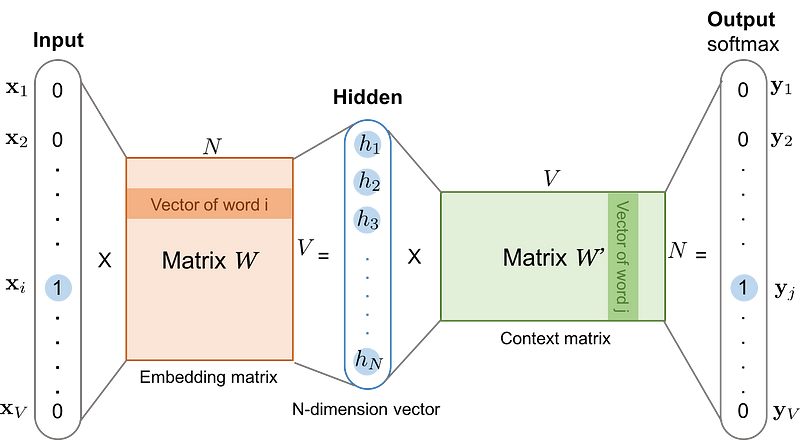
With colors and real word vectors
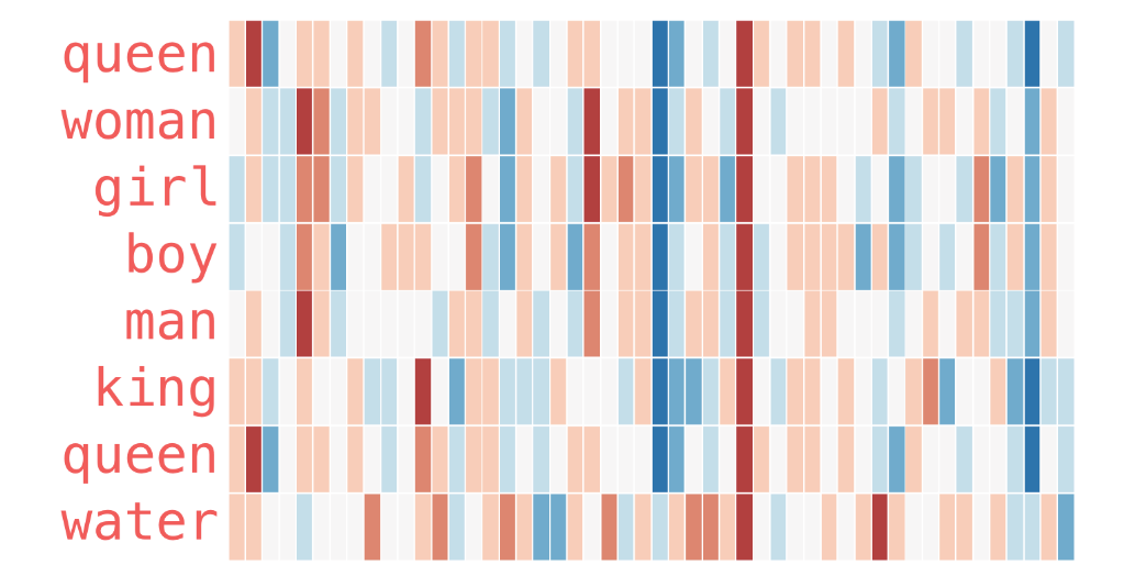
Source: Illustrated Word2Vec
Word Embeddings
Encoding similarity: vectors are not ortogonal anymore!
Automatic Generalization: learn about one word allow us to automatically learn about related words
Encodes Meaning: by learning the context, I can learn what a word means.
As a consequence:
Word Embeddings improves by ORDERS OF MAGNITUDE several Text-as-Data Tasks.
Allows to deal with unseen words.
Form the core idea of state-of-the-art models, such as LLMs.
Deep Learning for Text Analysis
Introduction to Deep Learning
Basics of Machine Learning
Deep Learning is a subfield of machine learning based on using neural networks models to learn.
As in any other statistical model, the goal of machine learning is to use data to learn about some output.
\[ y = f(X) + \epsilon\]
Where:
\(y\) is the outcome/dependent/response variable
\(X\) is a matrix of predictors/features/independent variables
\(f()\) is some fixed but unknown function mapping X to y. The “signal” in the data
\(\epsilon\) is some random error term. The “noise” in the data.
Linear models (OLS)
The simplest model we can use is an linear model (the classic OLS regression)
\[ y = b_0 + WX + \epsilon\]
Where:
- \(W\) is a vector of dimension p,
- \(X\) is the feature vector of dimension p
- \(b\) is a bias term (intercept)
Using Matrix Algebra
\[\mathbf{W} = \begin{bmatrix} w_1 & w_2 & \dots & w_p\end{bmatrix}\]
\[\mathbf{X} = \begin{bmatrix} X_1 \\ X_2 \\ X_3 \\ \vdots \\ X_p \end{bmatrix}\]
With matrix multiplication:
\[\mathbf{W} \mathbf{X} + b = w_1 X_1 + w_2 X_2 + \dots + w_p X_p + b\]
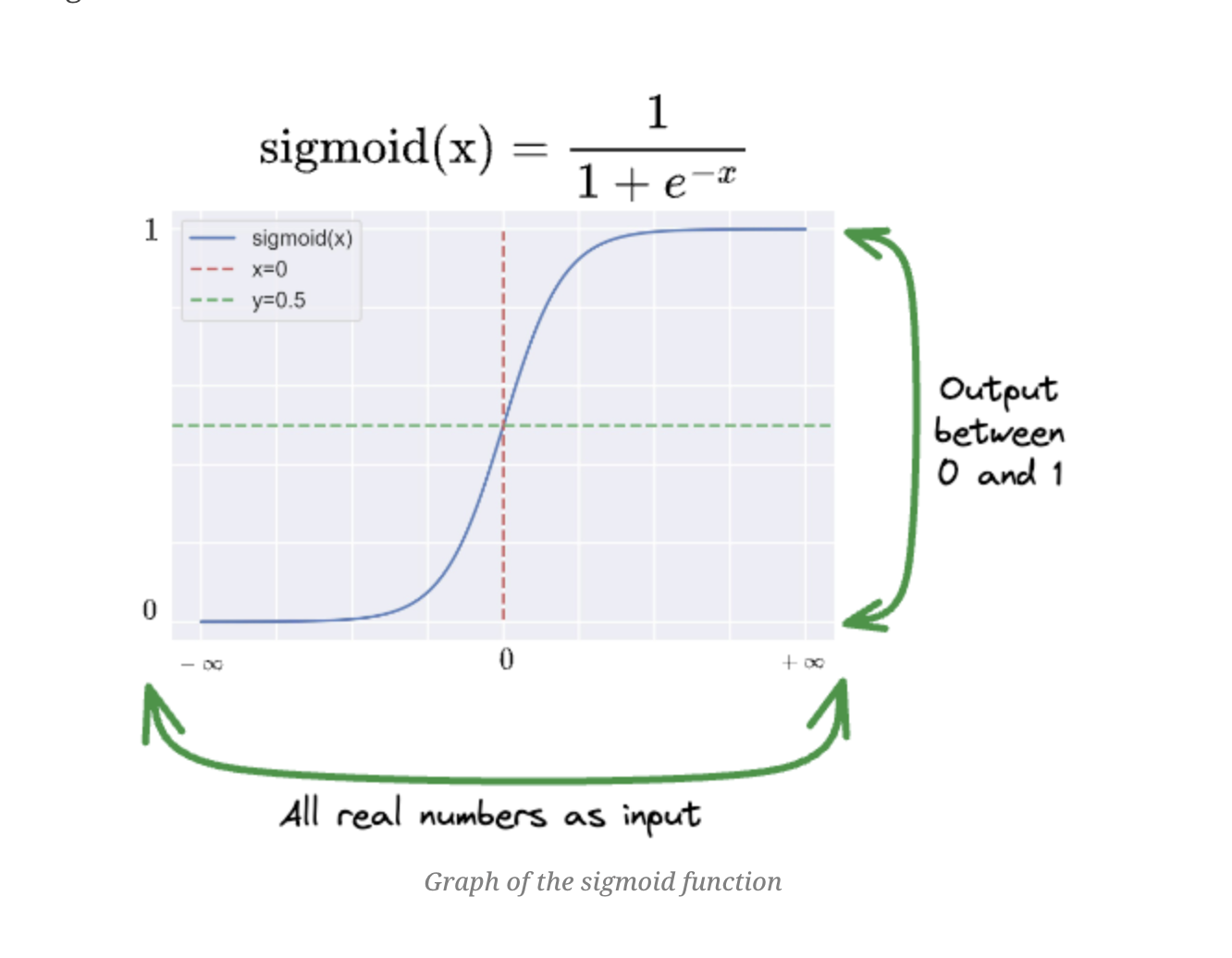
Logistic Regression
If we want to model some type of non-linearity, necessary for example when our outcome is binary, we can add a transformation function to make things non-linear:
\[ y = \sigma (b_0 + WX + \epsilon)\]
Where:
\[ \sigma(b_0 + WX + \epsilon) = \frac{1}{1 + \exp(-b_0 + WX + \epsilon)}\]
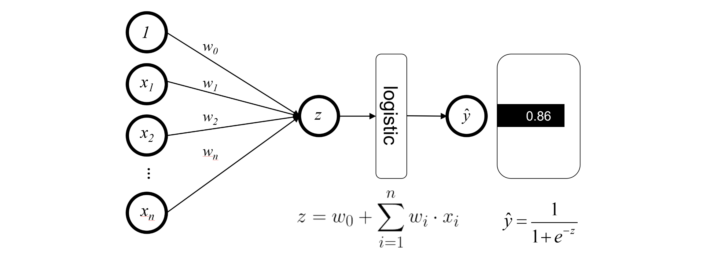
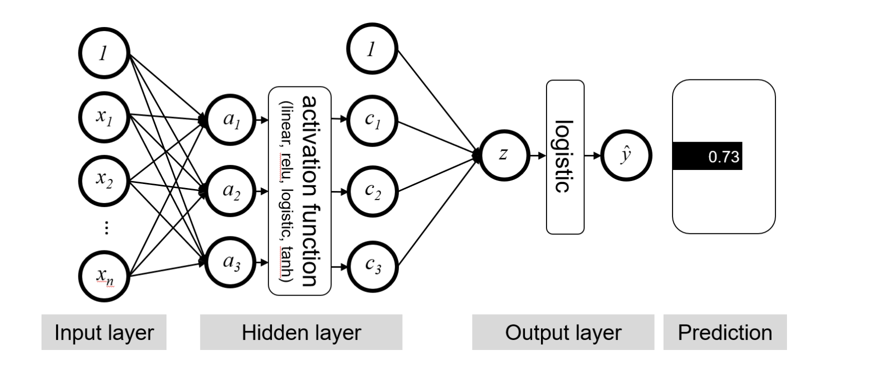
Logistic Regression as a Neural Network
Assume we have a simple model of voting. We want to predict if individual \(i\) will vote (\(y=1\)), and we will use four socio demographic factors to make this prediction.
Classic statistical approach with logistic regression:
\[ \hat{P(Y_i=1|X)} = \sigma(b_0 + WX + \epsilon) \]
We use MLE (Maximum Likelihood estimation) to find the parameters \(W\) and \(b_0\). We assume:
\[ Y_i \sim \text{Bernoulli}(\pi_i) \]
The likelihood function for \(n\) independent observations is:
\[L(W, b_0) = \prod_{i=1}^{n} \pi_i^{y_i} (1 - \pi_i)^{1 - y_i}.\]
The Famous: Cross-entropy loss functions
Take the log to make things easier:
\[-\ell(W, b_0) = - \sum_{i=1}^{n} \Big[ y_i \log(\pi_i) + (1 - y_i)\log(1 - \pi_i) \Big]\]
Where \(\pi_i\) = \(\sigma(b_0 + WX + \epsilon)\)
To solve this analytically:
take the derivative of \(\ell\) with respects to the parameter
set this equation to zero.
most times this solution will not exist, so we will use numerical approaches
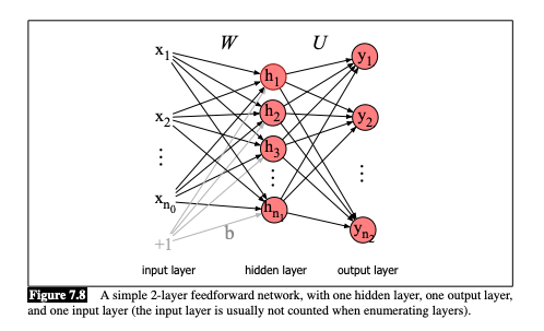
Neural Network Graphical Representation
Deep Neural Networks
A Deep Neural Network is equivalent to stacking multiple logistic regressions vertically and repeat this process multiple times across many layers.
As a Matrix, instead of:
\[\mathbf{W}_{previous} = \begin{bmatrix} w_1 & w_2 & \dots & w_p\end{bmatrix}\]
We use this set of parameters:
\[ \mathbf{W} = \begin{bmatrix} w_{11} & w_{12} & w_{13} & \dots & w_{1p} \\ w_{21} & w_{22} & w_{23} & \dots & w_{2p} \\ w_{31} & w_{32} & w_{33} & \dots & w_{3p} \\ \vdots & \vdots & \vdots & \vdots & \vdots \\ w_{k1} & w_{k2} & w_{k3} & \dots & w_{kp} \end{bmatrix} \]
Then, every line becomes a different logistic regression
\[\mathbf{WX} = \begin{bmatrix} \sigma(w_{11} X_1 + w_{12} X_2 + \dots + w_{1p}X_p) \\ \sigma(w_{21} X_1 + w_{22} X_2 + \dots + w_{2p}X_p) \\ \sigma(w_{31} X_1 + w_{32} X_2 + \dots + w_{3p}X_p )\\ \vdots \\ \sigma(w_{k1} X_1 + w_{k2} X_2 + \dots + w_{kp}X_p) \end{bmatrix}\] We then combine all of those with another set of parameters:
\[ \begin{align*} \mathbf{HA} &= h1 \cdot \sigma(w_{11} X_1 + w_{12} X_2 + \dots + w_{1p}X_p)\\ &+ h_2\cdot \sigma(w_{21} X_1 + w_{22} X_2 + \dots + w_{2p}X_p)\\ &+ h_3 \cdot \sigma (w_{31} X_1 + w_{32} X_2 + \dots + w_{3p}X_p)\\ &+ \dots + h_k + \sigma(w_{k1} X_1 + w_{k2} X_2 + \dots + w_{kp}X_p) \end{align*} \]
Feed Forward on a Deep Neural Network
Key Components
Input: p features (the original data) of an observation are linearly transformed into k1 features using a weight matrix of size k1×p
Embedding Matrices: Parameters you multiply your data by.
Neurons: Number of dimensions on your embedding matrices
Hidden Layer: the transformation that consists of the linear transformation and an activation function
Output Layer: the transformation that consists of the linear transformation and then (usually) a sigmoid (or some other activation function) to produce the final output predictions
Let’s take a step back!
Weights matrices are just parameters… the \(\beta_s\) of our regression models.
There are too MANY of them!! Neural Networks are a black box!
But… they also serve as way to project covariates (or words!) in a dense dimensional space.
Remember:
One-hot encoding / Sparse Representation:
cat = \(\begin{bmatrix} 0,0, 0, 0, 0, 0, 1, 0, 0 \end{bmatrix}\)
dog = \(\begin{bmatrix} 0,0, 0, 0, 0, 1, 0, 0, 0 \end{bmatrix}\)
Word Embedding / Dense Representation:
cat = \(\begin{bmatrix} 0.25, -0.75, 0.90, 0.12, -0.50, 0.33, 0.66, -0.88, 0.10, -0.45 \end{bmatrix}\)
dog = \(\begin{bmatrix} 0.25, 1.75, 0.90, 0.12, -0.50, 0.33, 0.66, -0.88, 0.10, -0.45 \end{bmatrix}\)
Deep Neural Network for Textual Data
Estimation: How do get good parameters?
To estimate the parameters, we will use a algorithm called gradient descent.
As in any other estimation approaches, we start with a loss function.
Loss function: used to measure how well or poorly a model is making predictions
The model makes a guess (prediction)
The loss function compares the guess to the correct answer (the actual data)
It then calculates the number that represents how “off” the answer was, which is the loss
The goal in training a model is to minimize this loss
Examples
Linear Regression: MSE
\[\text{RSS} = \sum_{i=1}^{n} (y_i - \widehat{y}_i)^2 \]
Logistic Regression: Negative Log Likelihood of a Bernoulli distribution
\[L(\beta) = -\sum_{i=1}^{n} \left( y_i \log(\widehat{y}_i) + (1-y_i)\log(1 - \widehat{y}_i) \right)\]
Fully-Connected Neural Network (Classification, Binary): Binary Cross Entropy
\[L(\mathbf{W}) = -\frac{1}{n}\sum_{i=1}^{n} \left( y_i \log(\widehat{y}_i) + (1-y_i)\log(1 - \widehat{y}_i) \right)\]
Quizz
Logistic Regression: Negative Log Likelihood of a Bernoulli distribution
\[L(\beta) = -\sum_{i=1}^{n} \left( y_i \log(\widehat{y}_i) + (1-y_i)\log(1 - \widehat{y}_i) \right)\]
1 - What happens when your label y = 1, and your model outputs 1 as the predicted value?
2 - What happens when your label y = 1, and your model outputs 0.02 as the predicted value?
Visualizing the loss
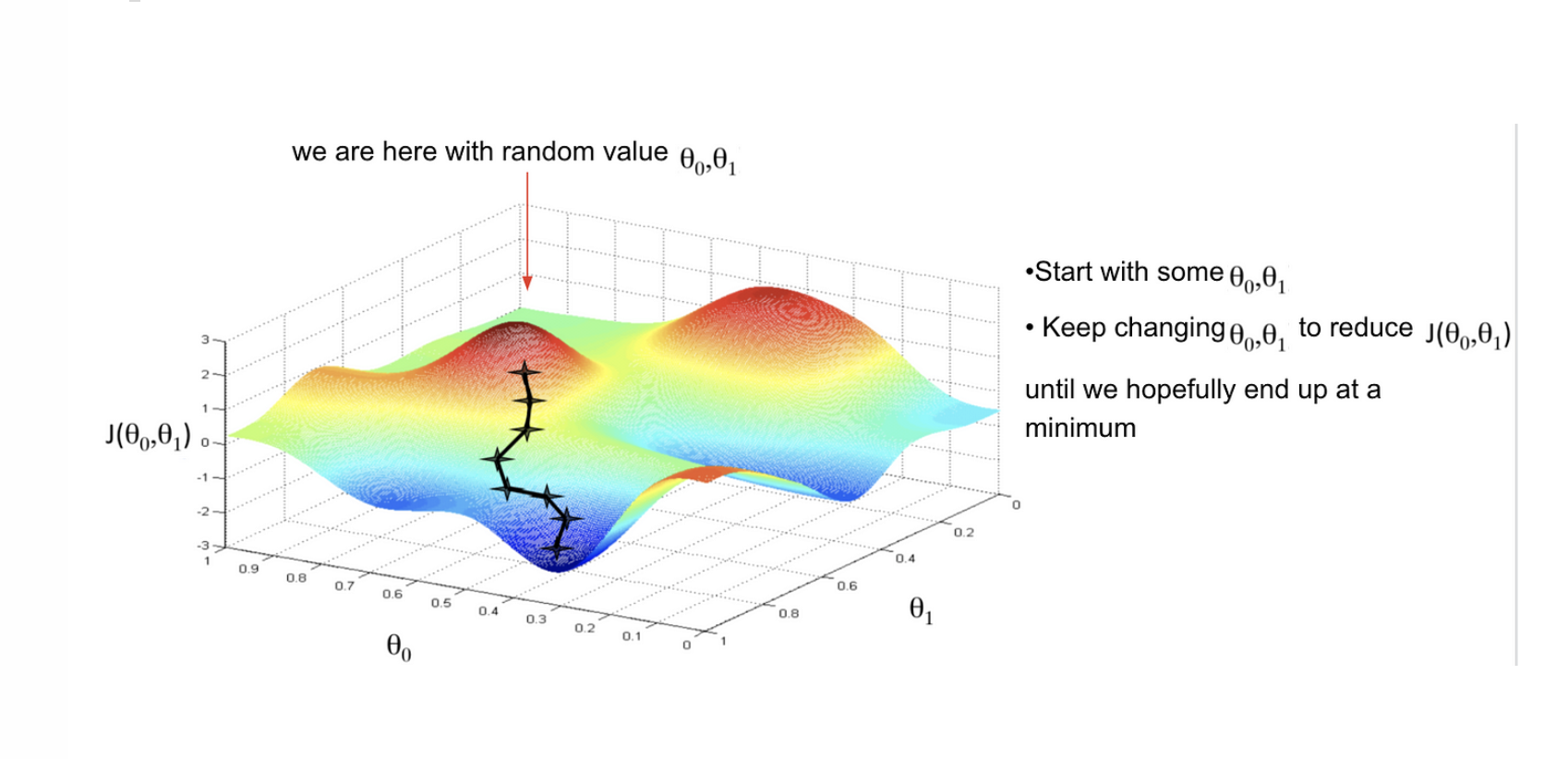
Updating parameters
Define a loss function
Gradient Descent Algorithm:
Initialize weights randomly
Feed Forward: Matrix Multiplication + Activation function
Get the loss for this iteration
Compute gradient (partial derivatives): \(\frac{\partial J(\mathbf{W})}{\partial \mathbf{W}}\)
Update weights: \(W_{new}: W_{old} -\eta \cdot \frac{\partial J(\mathbf{W})}{\partial \mathbf{W}}\)
Loop until convergence:
Let’s do some coding!
Text-as-Data