
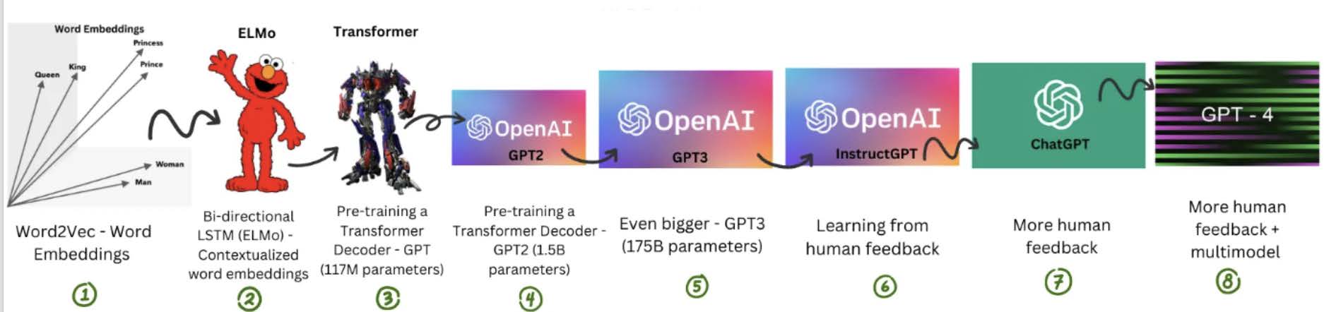
PPOL 6801 - Text as Data - Computational Linguistics
Week 9: Word Embeddings - Theory
Professor: Tiago Ventura
Plans for Today
Logistics: Replication
Word Embeddings
Semantics, Distributional Hypothesis, Moving from Sparse to Dense Vectors
Word2Vec Algorithm
Mathematical Model
Estimate with Neural Networks
Estimate using Co-Occurance matrices
In class exercise: How to select good embeddings?
Next week:
Coding
In class exercise about the readings (please do the readings!!)
Replication
Week 10: Presentation (This is all in the syllabus!)
You will do a presentation of your replication in two week.
Each group will have about 20 minutes (15 presentation + 5 Q&A)
You presentation should have the following sections:
Introduction: introduction summarizing the article.
Methods: data used in the article
Results: the results you were able to replicate
Differences: any differences between your results and the authors’
Autopsy of the replication: what did work and what did not work
Extension: what would you do differently if you were to write this article today? Where would you innovate?
EOW: Replication Repository
By Friday EOD of the replication week, you should share with me and all your colleagues (share on the slack channel) your replication report. The replication report should be:
a GitHub repo with a well-detailed readme. See a model here: https://github.com/TiagoVentura/winning_plosone
your presentation as a pdf
the code used in the replication as a notebook (Markdown or Jupyter)
a report with a maximum of 5 pages (it is fine if you do less than that) summarizing the replication process, with emphasis on four sections of your presentation: Results, Differences, Autopsy, and Extension.
Word Embeddings
Vector Space Model
In the vector space model, we learned:
A document \(D_i\) is represented as a collection of features \(W\) (words, tokens, n-grams..)
Each feature \(w_i\) can be place in a real line, then a document \(D_i\) is a point in a \(W\) dimensional space.
Embedded in this model, there is the idea we represent words as a one-hot encoding.
- “cat”: [0,0, 0, 0, 0, 0, 1, 0, ….., V] , on a V dimensional vector
- “dog”: [0,0, 0, 0, 0, 0, 0, 1, …., V], on a V dimensional vector
How can we embed some notion of meaning in the way we represent words?
Distributional Semantics
“you shall know a word by the company it keeps.” J. R. Firth 1957
Distributional semantics: words that are used in the same contexts tend to be similar in their meaning.
How can we use this insight to build a word representation?
Learn this representation from the unlabeled data.
Move from sparse representation to dense representation
Represent words as vectors of numbers with high number of dimensions
Each feature on this vectors embeds some information from the word
Why Word Embeddings?
Encoding similarity: vectors are not orthogonal anymore!
Encodes Meaning: by learning the context, I can somewhat learn what a word means.
Automatic Generalization: learn about one word allow us to automatically learn about related words
As a consequence:
Word Embeddings improves several NLP/Text-as-Data Tasks.
Allows to deal with unseen words.
Form the core idea of state-of-the-art models, such as LLMs.
Estimating Word Embeddings
Approches:
- Neural Networks: rely on the idea of self-supervision
- use unlabeled data and use words to predict sequence
- the famous word2vec algorithm
- Skipgram: predicts context words
- Continuous Bag of Words: predict center word
- Count-based methods: look at how often words co-occur with neighbors.
- Use this matrix, and use some factorization to retrieve vectors for the words
- Fast, not computationally intensive, but not the best representation, because it is not fully local
- This approach is somewhat implemented by the “GloVE” algorithm
Word2Vec: a framework for learning word vectors (Mikolov et al. 2013)
Developed in 2013 by Tomas Mikolov and colleagues at Google
Popular embedding method; fast to train, with pre-trained embeddings available online
Trained on large text corpora such as Google News (100 billion words), Wikipedia, and other massive datasets
Captures semantic information by learning how words appear in similar contexts
Represents word meaning based on surrounding words (context)
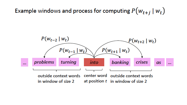
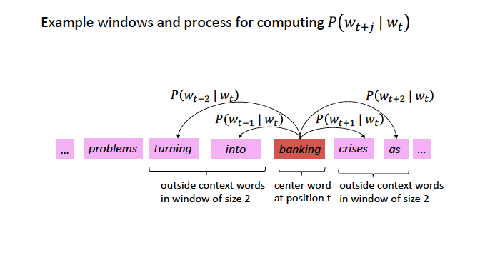
Word2Vec:Core Idea
We have a large corpus (“body”) of text: a long list of words
Every word in a fixed vocabulary is represented by a vector
Go through each position t in the text, which has a center word \(c\) and context (“outside”) words \(t\)
Use the similarity of the word vectors for \(c\) and \(t\) to calculate the probability of of t given c (or vice versa)
Keep adjusting the word vectors to maximize this probability
- Neural Network + Gradient Descent
Skipgram Example: Self-Supervision (Big Idea!)
Source: CS224N
Skigram Example: Self-Supervision
Source: CS224N
Encoding Similarity
To estimate the model, we first need to formalize the probability function we want to estimate.
This is similar to a logistic regression
In logistic regression: probability of a event occur given data X and parameters \(\beta\):
\[ P(y=1| X, \beta ) = X * \beta + \epsilon \]
\(X * \beta\) is not a proper probability function, so we make it to proper probability by using a logit transformation.
\(P(y=1|X, \beta ) = \frac{exp(XB)}{1 + exp(XB)}\)
Use transformation inside of a bernouilli distribution, get the likelihood function, and find the parameters using maximum likelihood estimation:
\[L(\beta) = \prod_{i=1}^n \bigl[\sigma(X_i^\top \beta)\bigr]^{y_i} \bigl[1 - \sigma(X_i^\top \beta)\bigr]^{1 - y_i} \]
\(P(w_t|w_{t-1})\)
This is the probability we want to estimate. To do so, we need to add parameters to it:
- \(P(w_t|w_{t-1})\) represents how similar these words are.
- The jump: if we assume words are vectors, we can estimate their similarities:
- \(P(w_t|w_{t-1}) = u_c \cdot u_t\)
- \(u_c \cdot u_t\)
- dot product between vectors (\(x_1*y_1 + x_2*y_2 .... x_n*y_n\))
- measures similarity using vector projection
- \(u_c\): center vector
- \(u_t\): target/neighbor vectors
- \(u_c \cdot u_t\) is also not a proper probability distribution. So we will use a softmax transformation.
\[P(w_t|w_{t-1}) = \frac{exp(u_c \cdot u_t)}{{\sum_{w}^V exp(u_c*u_w)}}\] - mathematically, this is the logistic transformation (sigmoid) for multiple classes.
Softmax Transformation
\[P(w_t|w_{t-1}) = \frac{exp(u_c \cdot u_t)}{{\sum_{w}^V exp(u_c*u_w)}}\]
Dot product compares similarity between vectors
numerator: center vs target vectors
exponentiation makes everything positive
Denominator: normalize over entire vocabulary to give probability distribution
What is the meaning of softmax?
max: assign high values to be 1
soft: still assigns some probability to smaller values
generalization of the logit ~ multinomial logistic function.
Skipgram Architecture
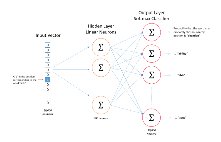
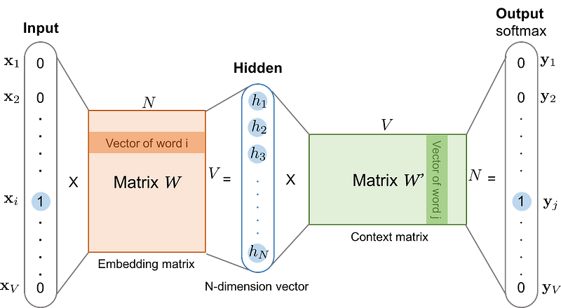
Training Word2Vec Step 1: learn the word embedding
Step 1: Compute Hidden Layer Representation
Input: A one-hot vector X where only the center word c has a value of 1, all others are 0 (size 1 x V)
Goal: Convert this into a dense vector of size D, where D is much smaller than the vocabulary size
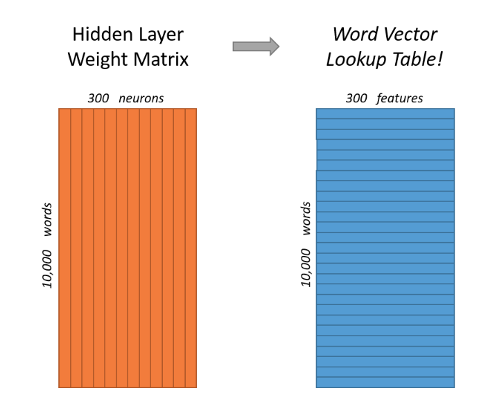
The word embedding matrix W has size V × D, where:
- V = vocabulary size (each row represents a word)
- D = embedding dimension (each column represents a dimension)
Multiplication XW:
- h = XW = (1 × V) × (V × D) = (1 × D)
This selects the i-th row of W, which is the word embedding for c
Example
Let’s practice with a vocabulary of size 5, a embedding with 3 dimensions, and the task is to predict ONLY the next word.
Step 1: v_{1,5} * W_{5,3} = C_{1,3}
- Where W is the embedding for center words
\[ \mathbf{v} = \begin{bmatrix} 0 \\ 0 \\ 1 \\ 0 \\ 0 \end{bmatrix} \]
\[ \mathbf{W} = \begin{bmatrix} .1 & .3 & -.23 \\ .2 & -.06 & -.26 \\ .3 & -.16& -.13 \\ .5 & .26 & -.03 \\ .6 & -.46 & -.53 \end{bmatrix} \]
\[v_T*W = C = \begin{bmatrix}.3 & -.16& -.13 \end{bmatrix} \]
Training Word2Vec Step 2: Compute Output Probabilities
Step 2 Goal: Predict which words are likely to appear near the center word
The hidden representation h = VtW is multiplied by a second weight matrix W′ (initialized randomly)
This produces a |V|-dimensional vector of unnormalized scores (logits), one for each word in the vocabulary. THIS IS A MEASURE FOR SIMILARITY FOR FREE!!
Compute the output scores (DOT Product between center and all other words!!!):
- u = hW′
Apply the softmax function to convert logits into probabilities:
The output probabilities indicate how likely each word is to appear in the context of the center word c
Example: Dot Product between vectors
Step 2: \(C_{1,3} * W2_{3,5} = P_{1,5}\)
- Where \(W_2\) is the embedding for context/target words
\[ C_{1,3} * W'_{3,5} = P_{1,5} \]
\[ \begin{bmatrix}.3 & -.16& -.13 \end{bmatrix} * \begin{bmatrix} .1 & .3 & -.23 & .3 & .5 \\ .2 & -.06 & -.26 & .3 & .5 \\ .3 & -.16& -.13 * .3 & .5\\ \end{bmatrix} \]
\[ P_{1,5}= \begin{bmatrix} -0.041 & 0.1204 & -0.02233 & -0.023 & 0.07 \end{bmatrix} \]
Take the softmax
\[ P(w_t|w_{t-1}) = \frac{exp(0.041)}{{exp(-0.041) + exp(0.1204) + exp(-0.02233) + exp(-0.023) + exp(0.07)}} \]
After that, you calculate the loss function with the negative likelihood (because you know which word you are predicting)
Use the loss to perform gradient descent and update the parameters
Word2Vec Skipgram: Loss function
For each position \(t\), predict context words within a window of fixed size \(m\), given center word \(w\).
Likelihood Function with Probabilities
\[ L= \prod_{t=1}^{T} \ \prod_{\substack{-m \leq j \leq m \\ j \neq 0}} P(w_{t+j}|w_t) \]
Likelihood Function
\[ L= \prod_{t=1}^{T} \ \prod_{\substack{-m \leq j \leq m \\ j \neq 0}} \frac{\exp\left( \mathbf{u}_{w_{t+j}}^\top \mathbf{v}_{w_t} \right)} {\sum_{w \in V} \exp\left( \mathbf{u}_w^\top \mathbf{v}_{w_t} \right)} \]
Log-Likelihood
\[ \log L= \sum_{t=1}^{T} \ \sum_{\substack{-m \leq j \leq m \\ j \neq 0}} \log \left( \frac{\exp\left( \mathbf{u}_{w_{t+j}}^\top \mathbf{v}_{w_t} \right)} {\sum_{w \in V} \exp\left( \mathbf{u}_w^\top \mathbf{v}_{w_t} \right)} \right) \]
Understanding the Loss Function
Negative Log-Likelihood + Decomposing the log
\[ -\log L = \sum_{t=1}^{T} \ \sum_{\substack{-m \leq j \leq m \\ j \neq 0}} \left[ - \mathbf{u}_{w_{t+j}}^\top \mathbf{v}_{w_t} + \log \sum_{w \in V} \exp\left( \mathbf{u}_w^\top \mathbf{v}_{w_t} \right) \right] \] First term: Rewards for assigning high probability to the correct word.
Second Term: Penalty for assigning high probabilities to other wrong words
Real Skipgram Algorithm

Word Embeddings Matrices
Skip-gram vs. CBOW: Neural Network Process
Step 1: Input
- SG: Take a single word as input
- CBOW: Take multiple words (context) as input
Step 2: Embedding Representation
- SG: Map it to its embedding vector (hidden layer weights)
- CBOW: Average their embeddings (combining hidden layer weights)
Step 3: Prediction
- SG: Predict multiple context words from this embedding.
- CBOW: Predict the target word using this averaged representation
Step 4: Loss Computation
- SG: Use softmax or negative sampling to compute loss.
- CBOW: Compute loss with softmax or negative sampling
Training Embeddings
Embeddings need quite a lot of text to train: e.g. want to disambiguate meanings from contexts. You can download pre-trained, or get the code and train locally
Word2Vec is trained on the Google News dataset (∼ 100B words, 2013)
GloVe are trained on different things: Wikipedia (2014) + Gigaword (6B words), Common Crawl, Twitter. And uses a mix of co-occurence matrix + local estimation instead of Neural Networks (More about that later today)
fastext from facebook
Word Embeddings Quiz
Explain these three concepts: Self-Supervision, Distributional Hypothesis, Dense Representation. And put these three concepts together to explain how word vectors can capture meaning of words.
What are the two main strategies to estimate word embeddings? One is named Glove, and the other is named Word2Vec
Are word embeddings still a bag-of-word representation model?
Are word2vec algorithms unsupervised or supervised learning?
Applications
Word Embeddings Decisions
When using/training embeddings, we face some key decisions:
Dimensionality: dimensions of the word vectors (50, 100, 300)
Window Size: how big of a window you want around the center word (5-10 good balance)
Minimum Count: how many times a word has to appear in the corpus for it to be assigned a vector (5 default in Word2Vec; for small, 1-3)
Model Type: Word2Vec (skip-gram or continuous bag-of-words), Glove vs Word2Vec, Fully Global with Matrix Factorization
Number of Iterations: number of iterations (epochs) over the corpus (5 common default; 10-20 useful for smaller datasets)
Decisions when using embeddings, Rodriguez and Spirling, 2022
Consider: Window size, Number of dimensions for the embedding matrix, Pre-trained vs locally fit variants, which algorithm to use between Glove and Word2Vec.
In class exercise
Work in 5 groups, to answer:
How do the authors evaluate performance (Turing Test)
Responses for each:
- Window size
- Number of dimensions
- Pre-Trained (Glove) vs Local Models
- Glove vs Word2Vec
Share your screen to show the graph with this result and explain it.
Word Embeddings via Count Based Methods (No Deep Learning)
Count Based Approaches
Count-based methods rely on word co-occurrence to learn embeddings:
Compute Unigram Probabilities: Measure how often each word appears in the corpus
Compute Word Co-occurrences: Count how often words appear together across the entire corpus
Calculate PMI (Pointwise Mutual Information): Measures how much more often two words co-occur than expected by chance
\[ PMI(\text{word}_1, \text{word}_2) = \log \frac{P(\text{word}_1, \text{word}_2)}{P(\text{word}_1) \, P(\text{word}_2)} \]
Construct a Co-occurrence Matrix: Store PMI values in a large word-by-word matrix
Apply Singular Value Decomposition (SVD): Reduce the matrix to extract meaningful lower-dimensional word vectors
SVD is a matrix factorization technique used in linear algebra and data science
Reduces dimensionality by identifying important patterns in data: splits the matrix into fundamental patterns (singular vectors), ranked by importance (singular values)
- Love this youtube video here: https://www.youtube.com/watch?v=vSczTbgc8Rc
Glove algorithm is a variation of this approach.
See you next week!
Text-as-Data