PPOL 5203 Data Science I: Foundations

Tidy Data and Joining Methods in Pandas

Tiago Ventura

---

In this Notebook we cover

This is our last notebook of data wrangling with Pandas. We will cover:

• Tidy Data
• Joining Methods in Pandas

import pandas as pd
import numpy as np

Tidy Data

Data can be organized in many different ways and can target many different concepts. Having an consistent and well-established procedure for data organization will make your workflow, faster, more efficient and less prone to errors.

On tasks related to data visualization and data wrangling, we will often try to organize our datasets following a tidy data format proposed by Hadley Wickham in his 2014 article.

Consider the following 4 ways to organize the same data (example pulled from R4DS).

Example 1

Country	Year	Cases	Population
Afghanistan	1999	745	19987071
Afghanistan	2000	2666	20595360
Brazil	1999	37737	172006362
Brazil	2000	80488	174504898
China	1999	212258	1272915272
China	2000	213766	1280428583

Example 2

country	year	type	count
Afghanistan	1999	cases	745
Afghanistan	1999	population	19987071
Afghanistan	2000	cases	2666
Afghanistan	2000	population	20595360
Brazil	1999	cases	37737
Brazil	1999	population	172006362

Example 3

country	year	rate
Afghanistan	1999	745/19987071
Afghanistan	2000	2666/20595360
Brazil	1999	37737/172006362
Brazil	2000	80488/174504898
China	1999	212258/1272915272
China	2000	213766/1280428583

Example 4

country	1999	2000
Afghanistan	745	2666
Brazil	37737	80488
China	212258	213766

country	1999	2000
Afghanistan	19987071	20595360
Brazil	172006362	174504898
China	1272915272	1280428583

**Of the data examples outlined above, only the first could be considered `tidy` by this definition.**

What makes a data tidy?

Three interrelated rules which make a dataset tidy:

1. Each variable must have its own column.

1. Each observation must have its own row.

1. Each value must have its own cell.

Why Tidy?

There are many reasons why tidy format facilitates data analysis:

• Facilitates split-apply-combine analysis
• Take full advantage of pandas vectorize operations over columns,
• Allows for apply operations over unit of your data
• Sits well with grammar of graphs approach for visualization

You don't need to be convinced in theory of these advantages. You will get in practice the taste of working with tidy format data **The most important thing for you to have now is to follow a consistent strategy to organize your datasets, and apply these procedures across the board!**

Using pandas to tidy your data.

Most often you will encounter untidy datasets. A huge portion of your time as a data scientist will consist on apply tidy procedures to your dataset before starting any analysis or modeling. Let's learn some pandas methods for it!

Let's first create every example of datasets we saw above

base_url = "https://github.com/byuidatascience/data4python4ds/raw/master/data-raw/"
table1 = pd.read_csv("{}table1/table1.csv".format(base_url))
table2 = pd.read_csv("{}table2/table2.csv".format(base_url))
table3 = pd.read_csv("{}table3/table3.csv".format(base_url))
table4a = pd.read_csv("{}table4a/table4a.csv".format(base_url), names=["country", "cases_1999", "cases_2000"] )
table4b = pd.read_csv("{}table4b/table4b.csv".format(base_url), names=["country", "population_1999", "poulation_2000"] )
table5 = pd.read_csv("{}table5/table5.csv".format(base_url), dtype = 'object')

# see
table1

	country	year	cases	population
0	Afghanistan	1999	745	19987071
1	Afghanistan	2000	2666	20595360
2	Brazil	1999	37737	172006362
3	Brazil	2000	80488	174504898
4	China	1999	212258	1272915272
5	China	2000	213766	1280428583

For most real analyses, you will need to resolve one of three common problems to tidy your data:

• One variable might be spread across multiple columns (pd.melt())

• One observation might be scattered across multiple rows (pd.pivot_table())

• A cell might contain weird/non-sensical/missing values.

We will focus on the first two cases, as the last requires a mix of data cleaning skills that are spread over different notebooks

pd.melt() from wide to long

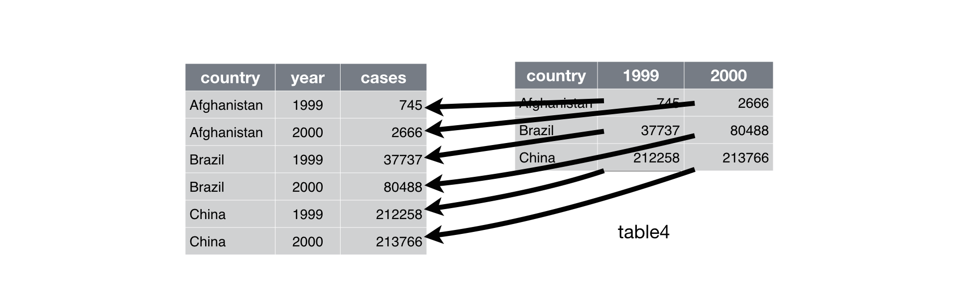
Requires:

• Columns whose names are identifier variables, and you wish to keep in the dataset as it is.

• A string for the new column with the variable names.

• A string for the new column with the values.

# untidy - wide
print(table4a)

       country  cases_1999  cases_2000
0      country        1999        2000
1  Afghanistan         745        2666
2       Brazil       37737       80488
3        China      212258      213766

# tidy - from wide to long
table4a.melt(id_vars=['country'], var_name = "year", value_name = "cases")

	country	year	cases
0	country	cases_1999	1999
1	Afghanistan	cases_1999	745
2	Brazil	cases_1999	37737
3	China	cases_1999	212258
4	country	cases_2000	2000
5	Afghanistan	cases_2000	2666
6	Brazil	cases_2000	80488
7	China	cases_2000	213766

help(pd.melt)

Help on function melt in module pandas.core.reshape.melt:

melt(frame: 'DataFrame', id_vars=None, value_vars=None, var_name=None, value_name='value', col_level=None, ignore_index: 'bool' = True) -> 'DataFrame'
    Unpivot a DataFrame from wide to long format, optionally leaving identifiers set.
    
    This function is useful to massage a DataFrame into a format where one
    or more columns are identifier variables (`id_vars`), while all other
    columns, considered measured variables (`value_vars`), are "unpivoted" to
    the row axis, leaving just two non-identifier columns, 'variable' and
    'value'.
    
    Parameters
    ----------
    id_vars : tuple, list, or ndarray, optional
        Column(s) to use as identifier variables.
    value_vars : tuple, list, or ndarray, optional
        Column(s) to unpivot. If not specified, uses all columns that
        are not set as `id_vars`.
    var_name : scalar
        Name to use for the 'variable' column. If None it uses
        ``frame.columns.name`` or 'variable'.
    value_name : scalar, default 'value'
        Name to use for the 'value' column.
    col_level : int or str, optional
        If columns are a MultiIndex then use this level to melt.
    ignore_index : bool, default True
        If True, original index is ignored. If False, the original index is retained.
        Index labels will be repeated as necessary.
    
        .. versionadded:: 1.1.0
    
    Returns
    -------
    DataFrame
        Unpivoted DataFrame.
    
    See Also
    --------
    DataFrame.melt : Identical method.
    pivot_table : Create a spreadsheet-style pivot table as a DataFrame.
    DataFrame.pivot : Return reshaped DataFrame organized
        by given index / column values.
    DataFrame.explode : Explode a DataFrame from list-like
            columns to long format.
    
    Notes
    -----
    Reference :ref:`the user guide <reshaping.melt>` for more examples.
    
    Examples
    --------
    >>> df = pd.DataFrame({'A': {0: 'a', 1: 'b', 2: 'c'},
    ...                    'B': {0: 1, 1: 3, 2: 5},
    ...                    'C': {0: 2, 1: 4, 2: 6}})
    >>> df
       A  B  C
    0  a  1  2
    1  b  3  4
    2  c  5  6
    
    >>> pd.melt(df, id_vars=['A'], value_vars=['B'])
       A variable  value
    0  a        B      1
    1  b        B      3
    2  c        B      5
    
    >>> pd.melt(df, id_vars=['A'], value_vars=['B', 'C'])
       A variable  value
    0  a        B      1
    1  b        B      3
    2  c        B      5
    3  a        C      2
    4  b        C      4
    5  c        C      6
    
    The names of 'variable' and 'value' columns can be customized:
    
    >>> pd.melt(df, id_vars=['A'], value_vars=['B'],
    ...         var_name='myVarname', value_name='myValname')
       A myVarname  myValname
    0  a         B          1
    1  b         B          3
    2  c         B          5
    
    Original index values can be kept around:
    
    >>> pd.melt(df, id_vars=['A'], value_vars=['B', 'C'], ignore_index=False)
       A variable  value
    0  a        B      1
    1  b        B      3
    2  c        B      5
    0  a        C      2
    1  b        C      4
    2  c        C      6
    
    If you have multi-index columns:
    
    >>> df.columns = [list('ABC'), list('DEF')]
    >>> df
       A  B  C
       D  E  F
    0  a  1  2
    1  b  3  4
    2  c  5  6
    
    >>> pd.melt(df, col_level=0, id_vars=['A'], value_vars=['B'])
       A variable  value
    0  a        B      1
    1  b        B      3
    2  c        B      5
    
    >>> pd.melt(df, id_vars=[('A', 'D')], value_vars=[('B', 'E')])
      (A, D) variable_0 variable_1  value
    0      a          B          E      1
    1      b          B          E      3
    2      c          B          E      5

pd.pivot_table() from long to wide (but tidy)

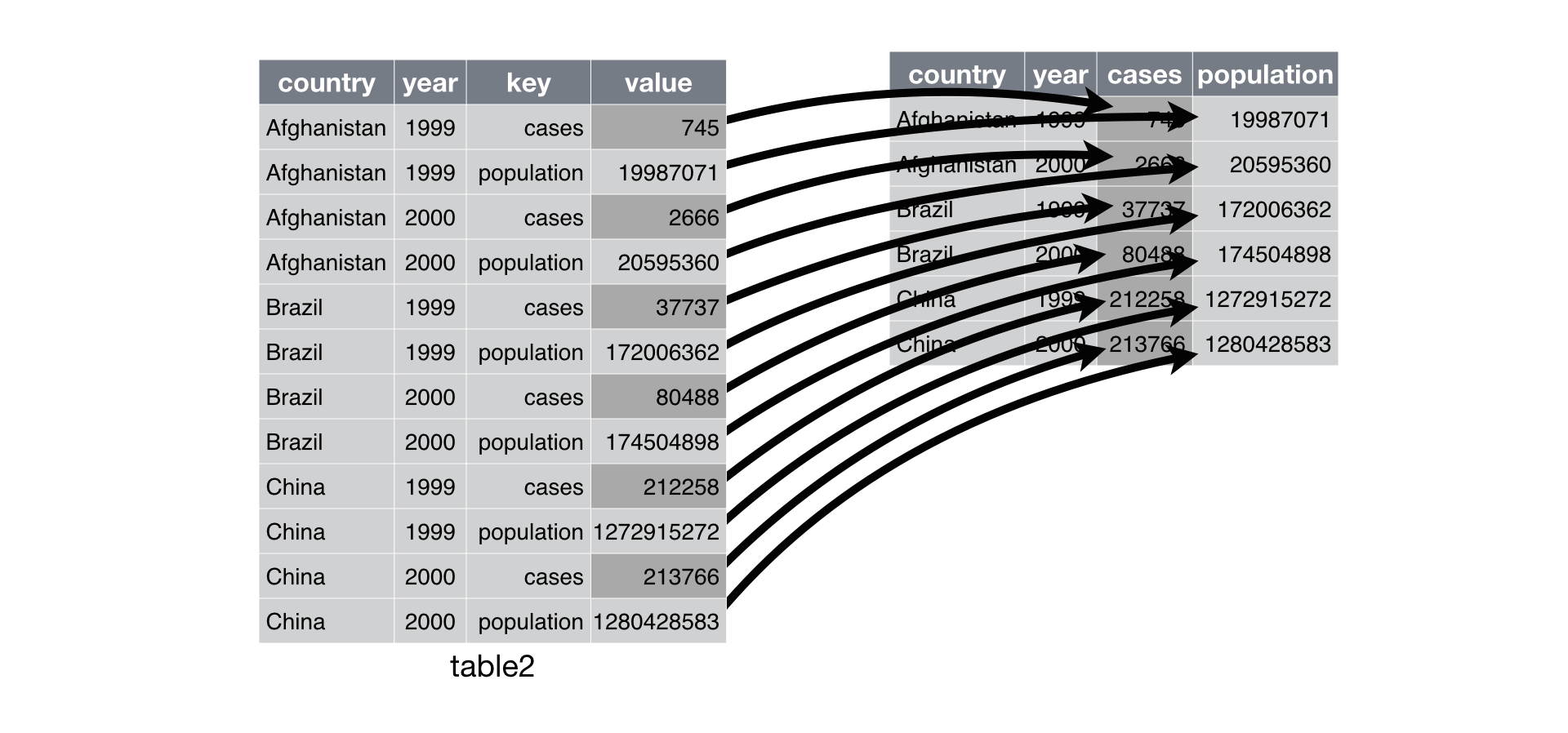
pivot_table() is the opposite of melt(). Think about this as you are widening a coarced variables. It requires:

• Index to hold your new dataset upon

• The column to open up across multiple new columnes.

• The column with the values to fill the cell on the new colum.

#untidy
print(table2)

        country  year        type       count
0   Afghanistan  1999       cases         745
1   Afghanistan  1999  population    19987071
2   Afghanistan  2000       cases        2666
3   Afghanistan  2000  population    20595360
4        Brazil  1999       cases       37737
5        Brazil  1999  population   172006362
6        Brazil  2000       cases       80488
7        Brazil  2000  population   174504898
8         China  1999       cases      212258
9         China  1999  population  1272915272
10        China  2000       cases      213766
11        China  2000  population  1280428583

#tidy
table2_tidy = table2.pivot_table(
    index = ['country', 'year'], 
    columns = 'type', 
    values = 'count')
# see
table2_tidy.reset_index()

type	country	year	cases	population
0	Afghanistan	1999	745	19987071
1	Afghanistan	2000	2666	20595360
2	Brazil	1999	37737	172006362
3	Brazil	2000	80488	174504898
4	China	1999	212258	1272915272
5	China	2000	213766	1280428583

help(pd.pivot_table)

Help on function pivot_table in module pandas.core.reshape.pivot:

pivot_table(data: 'DataFrame', values=None, index=None, columns=None, aggfunc: 'AggFuncType' = 'mean', fill_value=None, margins: 'bool' = False, dropna: 'bool' = True, margins_name: 'str' = 'All', observed: 'bool' = False, sort: 'bool' = True) -> 'DataFrame'
    Create a spreadsheet-style pivot table as a DataFrame.
    
    The levels in the pivot table will be stored in MultiIndex objects
    (hierarchical indexes) on the index and columns of the result DataFrame.
    
    Parameters
    ----------
    data : DataFrame
    values : column to aggregate, optional
    index : column, Grouper, array, or list of the previous
        If an array is passed, it must be the same length as the data. The
        list can contain any of the other types (except list).
        Keys to group by on the pivot table index.  If an array is passed,
        it is being used as the same manner as column values.
    columns : column, Grouper, array, or list of the previous
        If an array is passed, it must be the same length as the data. The
        list can contain any of the other types (except list).
        Keys to group by on the pivot table column.  If an array is passed,
        it is being used as the same manner as column values.
    aggfunc : function, list of functions, dict, default numpy.mean
        If list of functions passed, the resulting pivot table will have
        hierarchical columns whose top level are the function names
        (inferred from the function objects themselves)
        If dict is passed, the key is column to aggregate and value
        is function or list of functions.
    fill_value : scalar, default None
        Value to replace missing values with (in the resulting pivot table,
        after aggregation).
    margins : bool, default False
        Add all row / columns (e.g. for subtotal / grand totals).
    dropna : bool, default True
        Do not include columns whose entries are all NaN. If True,
        rows with a NaN value in any column will be omitted before
        computing margins.
    margins_name : str, default 'All'
        Name of the row / column that will contain the totals
        when margins is True.
    observed : bool, default False
        This only applies if any of the groupers are Categoricals.
        If True: only show observed values for categorical groupers.
        If False: show all values for categorical groupers.
    
        .. versionchanged:: 0.25.0
    
    sort : bool, default True
        Specifies if the result should be sorted.
    
        .. versionadded:: 1.3.0
    
    Returns
    -------
    DataFrame
        An Excel style pivot table.
    
    See Also
    --------
    DataFrame.pivot : Pivot without aggregation that can handle
        non-numeric data.
    DataFrame.melt: Unpivot a DataFrame from wide to long format,
        optionally leaving identifiers set.
    wide_to_long : Wide panel to long format. Less flexible but more
        user-friendly than melt.
    
    Notes
    -----
    Reference :ref:`the user guide <reshaping.pivot>` for more examples.
    
    Examples
    --------
    >>> df = pd.DataFrame({"A": ["foo", "foo", "foo", "foo", "foo",
    ...                          "bar", "bar", "bar", "bar"],
    ...                    "B": ["one", "one", "one", "two", "two",
    ...                          "one", "one", "two", "two"],
    ...                    "C": ["small", "large", "large", "small",
    ...                          "small", "large", "small", "small",
    ...                          "large"],
    ...                    "D": [1, 2, 2, 3, 3, 4, 5, 6, 7],
    ...                    "E": [2, 4, 5, 5, 6, 6, 8, 9, 9]})
    >>> df
         A    B      C  D  E
    0  foo  one  small  1  2
    1  foo  one  large  2  4
    2  foo  one  large  2  5
    3  foo  two  small  3  5
    4  foo  two  small  3  6
    5  bar  one  large  4  6
    6  bar  one  small  5  8
    7  bar  two  small  6  9
    8  bar  two  large  7  9
    
    This first example aggregates values by taking the sum.
    
    >>> table = pd.pivot_table(df, values='D', index=['A', 'B'],
    ...                     columns=['C'], aggfunc=np.sum)
    >>> table
    C        large  small
    A   B
    bar one    4.0    5.0
        two    7.0    6.0
    foo one    4.0    1.0
        two    NaN    6.0
    
    We can also fill missing values using the `fill_value` parameter.
    
    >>> table = pd.pivot_table(df, values='D', index=['A', 'B'],
    ...                     columns=['C'], aggfunc=np.sum, fill_value=0)
    >>> table
    C        large  small
    A   B
    bar one      4      5
        two      7      6
    foo one      4      1
        two      0      6
    
    The next example aggregates by taking the mean across multiple columns.
    
    >>> table = pd.pivot_table(df, values=['D', 'E'], index=['A', 'C'],
    ...                     aggfunc={'D': np.mean,
    ...                              'E': np.mean})
    >>> table
                    D         E
    A   C
    bar large  5.500000  7.500000
        small  5.500000  8.500000
    foo large  2.000000  4.500000
        small  2.333333  4.333333
    
    We can also calculate multiple types of aggregations for any given
    value column.
    
    >>> table = pd.pivot_table(df, values=['D', 'E'], index=['A', 'C'],
    ...                     aggfunc={'D': np.mean,
    ...                              'E': [min, max, np.mean]})
    >>> table
                      D   E
                   mean max      mean  min
    A   C
    bar large  5.500000   9  7.500000    6
        small  5.500000   9  8.500000    8
    foo large  2.000000   5  4.500000    4
        small  2.333333   6  4.333333    2

string methods with pandas

To tidy example three, we will use a combination of pandas and string methods. This combination will be around very often in our data cleaning tasks

# we need to separate rate
table3

	country	year	rate
0	Afghanistan	1999	745/19987071
1	Afghanistan	2000	2666/20595360
2	Brazil	1999	37737/172006362
3	Brazil	2000	80488/174504898
4	China	1999	212258/1272915272
5	China	2000	213766/1280428583

str.split(): to split strings in multiple elements

# simple string
hello, world = "hello/world".split("/")
print(hello)
print(world)

hello
world

# with pandas
table3[["cases","population"]]=table3['rate'].str.split("/",  expand=True)

table3

	country	year	rate	cases	population
0	Afghanistan	1999	745/19987071	745	19987071
1	Afghanistan	2000	2666/20595360	2666	20595360
2	Brazil	1999	37737/172006362	37737	172006362
3	Brazil	2000	80488/174504898	80488	174504898
4	China	1999	212258/1272915272	212258	1272915272
5	China	2000	213766/1280428583	213766	1280428583

string methods will be super helpful on cleaning your data

# all to upper
table3["country_upper"]=table3["country"].str.upper()

# length
table3["country_length"]=table3["country"].str.len()

# find 
table3["country_brazil_"]=table3["country"].str.find("Brazil")

# replace
table3["country_brazil"]=table3["country"].str.replace("Brazil", "BR")

# extract
table3[["century", "years"]] = table3["year"].astype(str).str.extract("(\d{2})(\d{2})")

# see all
table3

	country	year	rate	cases	population	country_upper	country_length	country_brazil_	country_brazil	century	years
0	Afghanistan	1999	745/19987071	745	19987071	AFGHANISTAN	11	-1	Afghanistan	19	99
1	Afghanistan	2000	2666/20595360	2666	20595360	AFGHANISTAN	11	-1	Afghanistan	20	00
2	Brazil	1999	37737/172006362	37737	172006362	BRAZIL	6	0	BR	19	99
3	Brazil	2000	80488/174504898	80488	174504898	BRAZIL	6	0	BR	20	00
4	China	1999	212258/1272915272	212258	1272915272	CHINA	5	-1	China	19	99
5	China	2000	213766/1280428583	213766	1280428583	CHINA	5	-1	China	20	00

Practice

Using both the World Cup Datasets from the Data Wrangling Notebook:

1. Select the following columns: MatchID, Year, Stage, Home Team Name, Away Team Name, Home Team Goals, Away Team Goals.

2. Clean the column names converting all to lower case and removing spaces.

3. Convert this data to the long format, having: a) a column indicating if the team played home or away, b) a single for the team

4. Which team have played more games in the history of the world cup?

5. Which team have played more games as home, and more games as away team?

# open datasets
wc = pd.read_csv("WorldCups.csv")
wc_matches = pd.read_csv("WorldCupMatches.csv")

# answer

Joining Methods

It is unlikely that your work as a data scientist will be restricted to analyze one isolated data frame -- or table in the SQL/Database lingo. Most often you have multiple tables of data, and your work will consist of combining them to answer the questions that you’re interested in.

There two major reasons for why complex datasets are often stored across multiple tables:

• A) Integrity and efficiency issues often referred as database normalization. As your data grow in size and complexity, keeping a unified database leads to redundancy and possible errors on data entry.

• B) Data comes from different sources. As a researcher, you are being creative and augmenting the information at your hand to answer a policy question.

Database normalization works as an **constraint**, a guardrail to protect your data infrastructure. The second reason for why joining methods matter is primarily an **opportunity** . Keep always your eyes open for creative ways to connect data sources. Very critical research ideas might emerge from data augmentation from joining unrelated datasets.

pandas methods:

pandas comes baked in with a fully functional method (pd.merge) to join data. However, we'll use the SQL language when talking about joins to stay consistent with SQL and R Tidyverse.

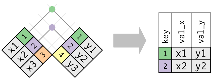
Let's start creating two tables for us to play around with pandas join methods

# Two fake data frames
import pandas as pd
data_x = pd.DataFrame(dict(key = ["1","2","3"],
                           var_x = ["x1","x2","x3"]))
data_y = pd.DataFrame(dict(key = ["1","2","4"],
                           var_y = ["y1","y2","y4"]))
display(data_x)
display(data_y)

	key	var_x
0	1	x1
1	2	x2
2	3	x3

	key	var_y
0	1	y1
1	2	y2
2	4	y4

Left Join: pd.merge(<data>, how="left")

• Keep all keys from the data set of the right

# chaining datasets
data_x.merge(data_y,how="left") 

	key	var_x	var_y
0	1	x1	y1
1	2	x2	y2
2	3	x3	NaN

# calling the construct
pd.merge(data_y, data_x,how="left")

	key	var_y	var_x
0	1	y1	x1
1	2	y2	x2
2	4	y4	NaN

Right Join: pd.merge(<data>, how="right")

• Keep all keys from the data set of the right

# chaining datasets
data_x.merge(data_y,how="right") 

	key	var_x	var_y
0	1	x1	y1
1	2	x2	y2
2	4	NaN	y4

Full (outer) Join: pd.merge(<data>, how="outer")

• Keep all keys from left and right

# chaining datasets
data_x.merge(data_y,how="outer") 

	key	var_x	var_y
0	1	x1	y1
1	2	x2	y2
2	3	x3	NaN
3	4	NaN	y4

Inner Join

• Keep only matched keys

# chaining datasets
data_x.merge(data_y,how="inner") 

	key	var_x	var_y
0	1	x1	y1
1	2	x2	y2

Handling disparate column names

# rename datasets
data_X = data_x.rename(columns={"key":"country_x"})
data_Y = data_y.rename(columns={"key":"country_y"})

# join now, and you will get an error
pd.merge(data_X,
         data_Y,
         how="left",
         left_on = "country_x",  # The left column naming convention 
         right_on="country_y") # The right column naming convention )

	country_x	var_x	country_y	var_y
0	1	x1	1	y1
1	2	x2	2	y2
2	3	x3	NaN	NaN

help(pd.merge)

Help on function merge in module pandas.core.reshape.merge:

merge(left: 'DataFrame | Series', right: 'DataFrame | Series', how: 'str' = 'inner', on: 'IndexLabel | None' = None, left_on: 'IndexLabel | None' = None, right_on: 'IndexLabel | None' = None, left_index: 'bool' = False, right_index: 'bool' = False, sort: 'bool' = False, suffixes: 'Suffixes' = ('_x', '_y'), copy: 'bool' = True, indicator: 'bool' = False, validate: 'str | None' = None) -> 'DataFrame'
    Merge DataFrame or named Series objects with a database-style join.
    
    A named Series object is treated as a DataFrame with a single named column.
    
    The join is done on columns or indexes. If joining columns on
    columns, the DataFrame indexes *will be ignored*. Otherwise if joining indexes
    on indexes or indexes on a column or columns, the index will be passed on.
    When performing a cross merge, no column specifications to merge on are
    allowed.
    
    .. warning::
    
        If both key columns contain rows where the key is a null value, those
        rows will be matched against each other. This is different from usual SQL
        join behaviour and can lead to unexpected results.
    
    Parameters
    ----------
    left : DataFrame
    right : DataFrame or named Series
        Object to merge with.
    how : {'left', 'right', 'outer', 'inner', 'cross'}, default 'inner'
        Type of merge to be performed.
    
        * left: use only keys from left frame, similar to a SQL left outer join;
          preserve key order.
        * right: use only keys from right frame, similar to a SQL right outer join;
          preserve key order.
        * outer: use union of keys from both frames, similar to a SQL full outer
          join; sort keys lexicographically.
        * inner: use intersection of keys from both frames, similar to a SQL inner
          join; preserve the order of the left keys.
        * cross: creates the cartesian product from both frames, preserves the order
          of the left keys.
    
          .. versionadded:: 1.2.0
    
    on : label or list
        Column or index level names to join on. These must be found in both
        DataFrames. If `on` is None and not merging on indexes then this defaults
        to the intersection of the columns in both DataFrames.
    left_on : label or list, or array-like
        Column or index level names to join on in the left DataFrame. Can also
        be an array or list of arrays of the length of the left DataFrame.
        These arrays are treated as if they are columns.
    right_on : label or list, or array-like
        Column or index level names to join on in the right DataFrame. Can also
        be an array or list of arrays of the length of the right DataFrame.
        These arrays are treated as if they are columns.
    left_index : bool, default False
        Use the index from the left DataFrame as the join key(s). If it is a
        MultiIndex, the number of keys in the other DataFrame (either the index
        or a number of columns) must match the number of levels.
    right_index : bool, default False
        Use the index from the right DataFrame as the join key. Same caveats as
        left_index.
    sort : bool, default False
        Sort the join keys lexicographically in the result DataFrame. If False,
        the order of the join keys depends on the join type (how keyword).
    suffixes : list-like, default is ("_x", "_y")
        A length-2 sequence where each element is optionally a string
        indicating the suffix to add to overlapping column names in
        `left` and `right` respectively. Pass a value of `None` instead
        of a string to indicate that the column name from `left` or
        `right` should be left as-is, with no suffix. At least one of the
        values must not be None.
    copy : bool, default True
        If False, avoid copy if possible.
    indicator : bool or str, default False
        If True, adds a column to the output DataFrame called "_merge" with
        information on the source of each row. The column can be given a different
        name by providing a string argument. The column will have a Categorical
        type with the value of "left_only" for observations whose merge key only
        appears in the left DataFrame, "right_only" for observations
        whose merge key only appears in the right DataFrame, and "both"
        if the observation's merge key is found in both DataFrames.
    
    validate : str, optional
        If specified, checks if merge is of specified type.
    
        * "one_to_one" or "1:1": check if merge keys are unique in both
          left and right datasets.
        * "one_to_many" or "1:m": check if merge keys are unique in left
          dataset.
        * "many_to_one" or "m:1": check if merge keys are unique in right
          dataset.
        * "many_to_many" or "m:m": allowed, but does not result in checks.
    
    Returns
    -------
    DataFrame
        A DataFrame of the two merged objects.
    
    See Also
    --------
    merge_ordered : Merge with optional filling/interpolation.
    merge_asof : Merge on nearest keys.
    DataFrame.join : Similar method using indices.
    
    Notes
    -----
    Support for specifying index levels as the `on`, `left_on`, and
    `right_on` parameters was added in version 0.23.0
    Support for merging named Series objects was added in version 0.24.0
    
    Examples
    --------
    >>> df1 = pd.DataFrame({'lkey': ['foo', 'bar', 'baz', 'foo'],
    ...                     'value': [1, 2, 3, 5]})
    >>> df2 = pd.DataFrame({'rkey': ['foo', 'bar', 'baz', 'foo'],
    ...                     'value': [5, 6, 7, 8]})
    >>> df1
        lkey value
    0   foo      1
    1   bar      2
    2   baz      3
    3   foo      5
    >>> df2
        rkey value
    0   foo      5
    1   bar      6
    2   baz      7
    3   foo      8
    
    Merge df1 and df2 on the lkey and rkey columns. The value columns have
    the default suffixes, _x and _y, appended.
    
    >>> df1.merge(df2, left_on='lkey', right_on='rkey')
      lkey  value_x rkey  value_y
    0  foo        1  foo        5
    1  foo        1  foo        8
    2  foo        5  foo        5
    3  foo        5  foo        8
    4  bar        2  bar        6
    5  baz        3  baz        7
    
    Merge DataFrames df1 and df2 with specified left and right suffixes
    appended to any overlapping columns.
    
    >>> df1.merge(df2, left_on='lkey', right_on='rkey',
    ...           suffixes=('_left', '_right'))
      lkey  value_left rkey  value_right
    0  foo           1  foo            5
    1  foo           1  foo            8
    2  foo           5  foo            5
    3  foo           5  foo            8
    4  bar           2  bar            6
    5  baz           3  baz            7
    
    Merge DataFrames df1 and df2, but raise an exception if the DataFrames have
    any overlapping columns.
    
    >>> df1.merge(df2, left_on='lkey', right_on='rkey', suffixes=(False, False))
    Traceback (most recent call last):
    ...
    ValueError: columns overlap but no suffix specified:
        Index(['value'], dtype='object')
    
    >>> df1 = pd.DataFrame({'a': ['foo', 'bar'], 'b': [1, 2]})
    >>> df2 = pd.DataFrame({'a': ['foo', 'baz'], 'c': [3, 4]})
    >>> df1
          a  b
    0   foo  1
    1   bar  2
    >>> df2
          a  c
    0   foo  3
    1   baz  4
    
    >>> df1.merge(df2, how='inner', on='a')
          a  b  c
    0   foo  1  3
    
    >>> df1.merge(df2, how='left', on='a')
          a  b  c
    0   foo  1  3.0
    1   bar  2  NaN
    
    >>> df1 = pd.DataFrame({'left': ['foo', 'bar']})
    >>> df2 = pd.DataFrame({'right': [7, 8]})
    >>> df1
        left
    0   foo
    1   bar
    >>> df2
        right
    0   7
    1   8
    
    >>> df1.merge(df2, how='cross')
       left  right
    0   foo      7
    1   foo      8
    2   bar      7
    3   bar      8

Concatenating by columns and rows

By Rows: pd.concat(<>, axis=0)

# full of NAS because the second columnes do not have the same name
pd.concat([data_x,data_y],
            sort=False) # keep the original structure

	key	var_x	var_y
0	1	x1	NaN
1	2	x2	NaN
2	3	x3	NaN
0	1	NaN	y1
1	2	NaN	y2
2	4	NaN	y4

By Columns: pd.concat(<>, axis=1)

pd.concat([data_x,data_y],axis=1)

	key	var_x	key	var_y
0	1	x1	1	y1
1	2	x2	2	y2
2	3	x3	4	y4

Note that when we row bind two DataFrame objects, pandas will preserve the indices. And you can use this to sort your dataset.

pd.concat([data_x,data_y],axis=0).sort_index()

	key	var_x	var_y
0	1	x1	NaN
0	1	NaN	y1
1	2	x2	NaN
1	2	NaN	y2
2	3	x3	NaN
2	4	NaN	y4

To keep the data tidy, we can preserve which data is coming from where by generating a hierarchical index using the key argument. Of course, this could also be done by creating a unique columns in each dataset before the join.

pd.concat([data_x,data_y],axis=0, keys=["data_x","data_y"])

		key	var_x	var_y
data_x	0	1	x1	NaN
	1	2	x2	NaN
	2	3	x3	NaN
data_y	0	1	NaN	y1
	1	2	NaN	y2
	2	4	NaN	y4

Lastly, note that we can completely ignore the index if need be.

pd.concat([data_x,data_y],axis=0,ignore_index=True)

	key	var_x	var_y
0	1	x1	NaN
1	2	x2	NaN
2	3	x3	NaN
3	1	NaN	y1
4	2	NaN	y2
5	4	NaN	y4

Practice

Using both the World Cup Datasets from the Data Wrangling Notebook:

1. Select the following columns: MatchID, Year, Stage, Home Team Name, Away Team Name, Home Team Goals, Away Team Goals.

2. Clean the column names converting all to lower case and removing spaces.

3. Convert this data to the long format, having: a) a single column for the teams playing; b) a single column for the goals scored.

4. Which team have the higher average of goals in the history of the world cup?

# open datasets
wc = pd.read_csv("WorldCups.csv")
wc_matches = pd.read_csv("WorldCupMatches.csv")

!jupyter nbconvert _week-5c-joining_data.ipynb --to html --template classic

[NbConvertApp] Converting notebook _week-5c-joining_data.ipynb to html
[NbConvertApp] Writing 367564 bytes to _week-5c-joining_data.html