PPOL 5203 Data Science I: Foundations

Data Wrangling in Pandas

Tiago Ventura


In this Notebook:

In this notebook, we will cover standard data wrangling methods using pandas:

  • Selecting Methods.
  • Filtering Methods.
  • Grouping and Summarization.
  • Recoding Variables.

Setup

In [91]:
import pandas as pd
import numpy as np

# set some options for pandas
pd.set_option('display.max_rows', 10)

Data Wrangling in pandas

Since you are also learning R throughout DSPP, let's provide you with an overview of the main Data Wrangling Functions in R using Tidyverse and Python using pandas.

Main (tidy) Data Wrangling Functions

pandas dplyr$^\dagger$ Description
.filter() select() select column variables/index
.drop() select() drop selected column variables/index
.rename() rename() rename column variables/index
.query() filter() row-wise subset of a data frame by a values of a column variable/index
.assign() mutate() Create a new variable on the existing data frame
.sort_values() arrange() Arrange all data values along a specified (set of) column variable(s)/indices
.groupby() group_by() Index data frame by specific (set of) column variable(s)/index value(s)
.agg() summarize() aggregate data by specific function rules
.pivot_table() spread() cast the data from a "long" to a "wide" format
pd.melt() gather() cast the data from a "wide" to a "long" format
.() %>% piping, fluid programming, or the passing one function output to the next

If you want to fully embrace the tidyverse style from R in Python, you should check the dfply module. This modules ofers an alternative to data wrangling in Python, and mirrors the popular tidyverse functionalities from R.

We will not cover dfply in class because I believe you should dominate pandas as data scientists that are fluent in Python. However, feel free to learn and even use in your homeworks and assignment.

In [93]:
# load worldcup datasets
wc = pd.read_csv("WorldCups.csv")
wc_matches = pd.read_csv("WorldCupMatches.csv")
In [94]:
# see wc data
wc.head()
Out[94]:
Year Country Winner Runners-Up Third Fourth GoalsScored QualifiedTeams MatchesPlayed Attendance
0 1930 Uruguay Uruguay Argentina USA Yugoslavia 70 13 18 590.549
1 1934 Italy Italy Czechoslovakia Germany Austria 70 16 17 363.000
2 1938 France Italy Hungary Brazil Sweden 84 15 18 375.700
3 1950 Brazil Uruguay Brazil Sweden Spain 88 13 22 1.045.246
4 1954 Switzerland Germany FR Hungary Austria Uruguay 140 16 26 768.607
In [95]:
# see matched data
wc_matches.head()
Out[95]:
Year Datetime Stage Stadium City Home Team Name Home Team Goals Away Team Goals Away Team Name Win conditions Attendance Half-time Home Goals Half-time Away Goals Referee Assistant 1 Assistant 2 RoundID MatchID Home Team Initials Away Team Initials
0 1930 13 Jul 1930 - 15:00 Group 1 Pocitos Montevideo France 4 1 Mexico 4444.0 3 0 LOMBARDI Domingo (URU) CRISTOPHE Henry (BEL) REGO Gilberto (BRA) 201 1096 FRA MEX
1 1930 13 Jul 1930 - 15:00 Group 4 Parque Central Montevideo USA 3 0 Belgium 18346.0 2 0 MACIAS Jose (ARG) MATEUCCI Francisco (URU) WARNKEN Alberto (CHI) 201 1090 USA BEL
2 1930 14 Jul 1930 - 12:45 Group 2 Parque Central Montevideo Yugoslavia 2 1 Brazil 24059.0 2 0 TEJADA Anibal (URU) VALLARINO Ricardo (URU) BALWAY Thomas (FRA) 201 1093 YUG BRA
3 1930 14 Jul 1930 - 14:50 Group 3 Pocitos Montevideo Romania 3 1 Peru 2549.0 1 0 WARNKEN Alberto (CHI) LANGENUS Jean (BEL) MATEUCCI Francisco (URU) 201 1098 ROU PER
4 1930 15 Jul 1930 - 16:00 Group 1 Parque Central Montevideo Argentina 1 0 France 23409.0 0 0 REGO Gilberto (BRA) SAUCEDO Ulises (BOL) RADULESCU Constantin (ROU) 201 1085 ARG FRA

Piping

If you started your data science career, or are simultaneously learning R, it is likely you were exposed to the tidyverse world, and the famous pipe. Here it is for you:

Pipe operators, introduced by tha magritt package in R, absolutely transformed the way of writing coding in R. It did for good reasons. And in the past few years, piping has also become more prevalent in Python.

Pipe operators allows you to:

  • Chain together data manipulations in a single operational sequence.

In pandas, piping allows you to chain together in a single workflow a sequence of methods. Pipe operators (.pipe()) in pandas were introduced relatively recently (version 0.16.2).

Let's see some examples using the world cup data. We want to count which country played more world cup games.

In [22]:
# read world cup data
#wc = pd.read_csv("WorldCupMatches.csv")

Method 1: sequentially overwrite the object

In [96]:
wc = pd.read_csv("WorldCupMatches.csv")

# select columns
wc = wc.filter(['Year','Home Team Name','Away Team Name'])

# make it tidy
wc = wc.melt(id_vars=["Year"], var_name="var", value_name="country")

# group by
wc = wc.groupby("country")

# count occurrences
wc = wc.size()

# move index to column with new name
wc = wc.reset_index(name="n")

# sort
wc = wc.sort_values(by="n", ascending=False)

# print 10
wc.head(10)
Out[96]:
country n
7 Brazil 108
39 Italy 83
2 Argentina 81
25 England 62
29 Germany FR 62
26 France 61
66 Spain 59
45 Mexico 54
47 Netherlands 54
74 Uruguay 52

Method 2: Pandas Pipe

In [99]:
wc = pd.read_csv("WorldCupMatches.csv")

# select columns
wc_10 = ( # encapsulate
            wc.filter(['Year','Home Team Name','Away Team Name']).
             melt(id_vars=["Year"], var_name="var", value_name="country"). 
             groupby("country"). 
             size(). 
             reset_index(name="n").
             sort_values(by="n", ascending=False)
        ) # close

# print 10
wc_10.head(10)
Out[99]:
country
Algeria       14
Angola         3
Argentina     81
Australia     13
Austria       29
Belgium       43
Bolivia        6
Brazil       108
Bulgaria      26
Cameroon      23
dtype: int64

Final notes in Piping

To understand pipes, you should always remember: **data in, data out**. That's what pipes do: apply methods sequentially to `pandas dataframes`.

It should be clear by now, but these are some of the advantages of piping your code:

  • Improves code structure
  • Eliminates intermediate variables
  • Can improve code readability
  • Memory efficiency by eliminating intermediate variables
  • Makes easier to add steps anywhere in the sequence of operations

Keep in mind pipes also have some disadvantages. In my view, specially when working in notebook in which you do not execute line by line, pipes can make codes a bit harder to debug and also embed errors that could be more easily perceived by examining intermediate variables.

Column-Wise Operations

For data wrangling tasks at the columns of your data frame, we will discuss:

  • Select columns
  • Drop columns
  • Create new columns
  • Rename columns

For all operations we will see index vs function-based implementation

Select Columns

Functionality:

  • Select specific variables/column indices

Implementation

  • Traditional indexing in pandas
  • .loc() methods
  • pd.filter() methods (allows piping).

Select via index

In [100]:
# load worldcup dataset
wc = pd.read_csv("WorldCups.csv")
wc_matches = pd.read_csv("WorldCupMatches.csv")
In [101]:
## simple index for columns
wc["Year"]
Out[101]:
0     1930
1     1934
2     1938
3     1950
4     1954
      ... 
15    1998
16    2002
17    2006
18    2010
19    2014
Name: Year, Length: 20, dtype: int64
In [102]:
## using dot method
wc.Year
Out[102]:
0     1930
1     1934
2     1938
3     1950
4     1954
      ... 
15    1998
16    2002
17    2006
18    2010
19    2014
Name: Year, Length: 20, dtype: int64
In [103]:
## using .loc method
wc.loc[:,"Year"]
Out[103]:
0     1930
1     1934
2     1938
3     1950
4     1954
      ... 
15    1998
16    2002
17    2006
18    2010
19    2014
Name: Year, Length: 20, dtype: int64

Notice, in all cases, the output comes as a pandas series. If you would like the output to be a full data frame, or if you need to select multiple columns, you should give a list of indexes as inputs

In [105]:
wc[["Winner","Year"]]
Out[105]:
Winner Year
0 Uruguay 1930
1 Italy 1934
2 Italy 1938
3 Uruguay 1950
4 Germany FR 1954
... ... ...
15 France 1998
16 Brazil 2002
17 Italy 2006
18 Spain 2010
19 Germany 2014

20 rows × 2 columns

.loc() methods for selecting columns

It allows you to select multible variables in between column names!

In [106]:
# .loc for a single or multiple columns
wc.loc[: , "Year":"Winner"]
Out[106]:
Year Country Winner
0 1930 Uruguay Uruguay
1 1934 Italy Italy
2 1938 France Italy
3 1950 Brazil Uruguay
4 1954 Switzerland Germany FR
... ... ... ...
15 1998 France France
16 2002 Korea/Japan Brazil
17 2006 Germany Italy
18 2010 South Africa Spain
19 2014 Brazil Germany

20 rows × 3 columns

In [107]:
# iloc for numeric positions
wc.iloc[0:10,0:3]
Out[107]:
Year Country Winner
0 1930 Uruguay Uruguay
1 1934 Italy Italy
2 1938 France Italy
3 1950 Brazil Uruguay
4 1954 Switzerland Germany FR
5 1958 Sweden Brazil
6 1962 Chile Brazil
7 1966 England England
8 1970 Mexico Brazil
9 1974 Germany Germany FR

.filter() method

The filter methods in Pandas works similarly to the select function in the Tidyverse in R. It has the following advantages:

  • Allows for a piping approach
  • Can be combined with regex queries for selectins columns
In [108]:
# simple filter
wc.filter(["Year", "Winner"])
Out[108]:
Year Winner
0 1930 Uruguay
1 1934 Italy
2 1938 Italy
3 1950 Uruguay
4 1954 Germany FR
... ... ...
15 1998 France
16 2002 Brazil
17 2006 Italy
18 2010 Spain
19 2014 Germany

20 rows × 2 columns

Using the like parameter: Select columns that contain a specific substring.

In [109]:
# like parameter. In R: data %>% select(contains("Away"))
wc_matches.filter(like="Away")
Out[109]:
Away Team Goals Away Team Name Half-time Away Goals Away Team Initials
0 1 Mexico 0 MEX
1 0 Belgium 0 BEL
2 1 Brazil 0 BRA
3 1 Peru 0 PER
4 0 France 0 FRA
... ... ... ... ...
847 0 Costa Rica 0 CRC
848 7 Germany 5 GER
849 0 Argentina 0 ARG
850 3 Netherlands 2 NED
851 0 Argentina 0 ARG

852 rows × 4 columns

Using the Regex: You can also input regex queries for selecting columns. More and More flexibility

In [110]:
# starts with
wc_matches.filter(regex="^Away")
Out[110]:
Away Team Goals Away Team Name Away Team Initials
0 1 Mexico MEX
1 0 Belgium BEL
2 1 Brazil BRA
3 1 Peru PER
4 0 France FRA
... ... ... ...
847 0 Costa Rica CRC
848 7 Germany GER
849 0 Argentina ARG
850 3 Netherlands NED
851 0 Argentina ARG

852 rows × 3 columns

In [111]:
# ends with
wc_matches.filter(regex="Initials$")
Out[111]:
Home Team Initials Away Team Initials
0 FRA MEX
1 USA BEL
2 YUG BRA
3 ROU PER
4 ARG FRA
... ... ...
847 NED CRC
848 BRA GER
849 NED ARG
850 BRA NED
851 GER ARG

852 rows × 2 columns

Drop Columns

Functionality:

Drop specific variables/column indices

Implementation:

  • Indexing + Boolean operations
  • .loc() methods
  • pd.drop() methods (allows piping).
In [112]:
## select all but "Year" and "Country"
wc[wc.columns[~wc.columns.isin(["Year", "Country"])]]
Out[112]:
Winner Runners-Up Third Fourth GoalsScored QualifiedTeams MatchesPlayed Attendance
0 Uruguay Argentina USA Yugoslavia 70 13 18 590.549
1 Italy Czechoslovakia Germany Austria 70 16 17 363.000
2 Italy Hungary Brazil Sweden 84 15 18 375.700
3 Uruguay Brazil Sweden Spain 88 13 22 1.045.246
4 Germany FR Hungary Austria Uruguay 140 16 26 768.607
... ... ... ... ... ... ... ... ...
15 France Brazil Croatia Netherlands 171 32 64 2.785.100
16 Brazil Germany Turkey Korea Republic 161 32 64 2.705.197
17 Italy France Germany Portugal 147 32 64 3.359.439
18 Spain Netherlands Germany Uruguay 145 32 64 3.178.856
19 Germany Argentina Netherlands Brazil 171 32 64 3.386.810

20 rows × 8 columns

In [113]:
# Indexing: Bit too much?!
# .isin returns a boolean.
wc.columns[~wc.columns.isin(["Year", "Country"])]
Out[113]:
Index(['Winner', 'Runners-Up', 'Third', 'Fourth', 'GoalsScored',
       'QualifiedTeams', 'MatchesPlayed', 'Attendance'],
      dtype='object')
In [114]:
# What is going on here?
~wc.columns.isin(["Year", "Country"])
Out[114]:
array([False, False,  True,  True,  True,  True,  True,  True,  True,
        True])
bol_col is an array of booleans. If you throw them directly as a index, Pandas interprets `wc[bol_col]` as trying to index the rows of the DataFrame, not the columns. This is because when you pass a boolean array directly to the DataFrame indexing operator [], pandas assumes you're trying to index rows based on the boolean array.
In [115]:
# loc methods
wc.loc[:,~wc.columns.isin(["Year", "Country"])]
Out[115]:
Winner Runners-Up Third Fourth GoalsScored QualifiedTeams MatchesPlayed Attendance
0 Uruguay Argentina USA Yugoslavia 70 13 18 590.549
1 Italy Czechoslovakia Germany Austria 70 16 17 363.000
2 Italy Hungary Brazil Sweden 84 15 18 375.700
3 Uruguay Brazil Sweden Spain 88 13 22 1.045.246
4 Germany FR Hungary Austria Uruguay 140 16 26 768.607
... ... ... ... ... ... ... ... ...
15 France Brazil Croatia Netherlands 171 32 64 2.785.100
16 Brazil Germany Turkey Korea Republic 161 32 64 2.705.197
17 Italy France Germany Portugal 147 32 64 3.359.439
18 Spain Netherlands Germany Uruguay 145 32 64 3.178.856
19 Germany Argentina Netherlands Brazil 171 32 64 3.386.810

20 rows × 8 columns

In [119]:
# indexing -> error
bol_col = ~wc.columns.isin(["Year", "Country"])
bol_col
wc[bol_col]
---------------------------------------------------------------------------
ValueError                                Traceback (most recent call last)
Cell In[119], line 4
      2 bol_col = ~wc.columns.isin(["Year", "Country"])
      3 bol_col
----> 4 wc[bol_col]

File ~/anaconda3/lib/python3.11/site-packages/pandas/core/frame.py:3798, in DataFrame.__getitem__(self, key)
   3796 # Do we have a (boolean) 1d indexer?
   3797 if com.is_bool_indexer(key):
-> 3798     return self._getitem_bool_array(key)
   3800 # We are left with two options: a single key, and a collection of keys,
   3801 # We interpret tuples as collections only for non-MultiIndex
   3802 is_single_key = isinstance(key, tuple) or not is_list_like(key)

File ~/anaconda3/lib/python3.11/site-packages/pandas/core/frame.py:3845, in DataFrame._getitem_bool_array(self, key)
   3839     warnings.warn(
   3840         "Boolean Series key will be reindexed to match DataFrame index.",
   3841         UserWarning,
   3842         stacklevel=find_stack_level(),
   3843     )
   3844 elif len(key) != len(self.index):
-> 3845     raise ValueError(
   3846         f"Item wrong length {len(key)} instead of {len(self.index)}."
   3847     )
   3849 # check_bool_indexer will throw exception if Series key cannot
   3850 # be reindexed to match DataFrame rows
   3851 key = check_bool_indexer(self.index, key)

ValueError: Item wrong length 10 instead of 20.
In [120]:
# With .loc, it works
wc.loc[:,bol_col]
Out[120]:
Winner Runners-Up Third Fourth GoalsScored QualifiedTeams MatchesPlayed Attendance
0 Uruguay Argentina USA Yugoslavia 70 13 18 590.549
1 Italy Czechoslovakia Germany Austria 70 16 17 363.000
2 Italy Hungary Brazil Sweden 84 15 18 375.700
3 Uruguay Brazil Sweden Spain 88 13 22 1.045.246
4 Germany FR Hungary Austria Uruguay 140 16 26 768.607
... ... ... ... ... ... ... ... ...
15 France Brazil Croatia Netherlands 171 32 64 2.785.100
16 Brazil Germany Turkey Korea Republic 161 32 64 2.705.197
17 Italy France Germany Portugal 147 32 64 3.359.439
18 Spain Netherlands Germany Uruguay 145 32 64 3.178.856
19 Germany Argentina Netherlands Brazil 171 32 64 3.386.810

20 rows × 8 columns

pd.drop() methods: easier way to go

In [121]:
wc.drop(columns=["Year"])
Out[121]:
Country Winner Runners-Up Third Fourth GoalsScored QualifiedTeams MatchesPlayed Attendance
0 Uruguay Uruguay Argentina USA Yugoslavia 70 13 18 590.549
1 Italy Italy Czechoslovakia Germany Austria 70 16 17 363.000
2 France Italy Hungary Brazil Sweden 84 15 18 375.700
3 Brazil Uruguay Brazil Sweden Spain 88 13 22 1.045.246
4 Switzerland Germany FR Hungary Austria Uruguay 140 16 26 768.607
... ... ... ... ... ... ... ... ... ...
15 France France Brazil Croatia Netherlands 171 32 64 2.785.100
16 Korea/Japan Brazil Germany Turkey Korea Republic 161 32 64 2.705.197
17 Germany Italy France Germany Portugal 147 32 64 3.359.439
18 South Africa Spain Netherlands Germany Uruguay 145 32 64 3.178.856
19 Brazil Germany Argentina Netherlands Brazil 171 32 64 3.386.810

20 rows × 9 columns

In [122]:
# see here why you need the argument columns
help(pd.DataFrame.drop)
Help on function drop in module pandas.core.frame:

drop(self, labels: 'IndexLabel' = None, *, axis: 'Axis' = 0, index: 'IndexLabel' = None, columns: 'IndexLabel' = None, level: 'Level' = None, inplace: 'bool' = False, errors: 'IgnoreRaise' = 'raise') -> 'DataFrame | None'
    Drop specified labels from rows or columns.
    
    Remove rows or columns by specifying label names and corresponding
    axis, or by specifying directly index or column names. When using a
    multi-index, labels on different levels can be removed by specifying
    the level. See the `user guide <advanced.shown_levels>`
    for more information about the now unused levels.
    
    Parameters
    ----------
    labels : single label or list-like
        Index or column labels to drop. A tuple will be used as a single
        label and not treated as a list-like.
    axis : {0 or 'index', 1 or 'columns'}, default 0
        Whether to drop labels from the index (0 or 'index') or
        columns (1 or 'columns').
    index : single label or list-like
        Alternative to specifying axis (``labels, axis=0``
        is equivalent to ``index=labels``).
    columns : single label or list-like
        Alternative to specifying axis (``labels, axis=1``
        is equivalent to ``columns=labels``).
    level : int or level name, optional
        For MultiIndex, level from which the labels will be removed.
    inplace : bool, default False
        If False, return a copy. Otherwise, do operation
        inplace and return None.
    errors : {'ignore', 'raise'}, default 'raise'
        If 'ignore', suppress error and only existing labels are
        dropped.
    
    Returns
    -------
    DataFrame or None
        DataFrame without the removed index or column labels or
        None if ``inplace=True``.
    
    Raises
    ------
    KeyError
        If any of the labels is not found in the selected axis.
    
    See Also
    --------
    DataFrame.loc : Label-location based indexer for selection by label.
    DataFrame.dropna : Return DataFrame with labels on given axis omitted
        where (all or any) data are missing.
    DataFrame.drop_duplicates : Return DataFrame with duplicate rows
        removed, optionally only considering certain columns.
    Series.drop : Return Series with specified index labels removed.
    
    Examples
    --------
    >>> df = pd.DataFrame(np.arange(12).reshape(3, 4),
    ...                   columns=['A', 'B', 'C', 'D'])
    >>> df
       A  B   C   D
    0  0  1   2   3
    1  4  5   6   7
    2  8  9  10  11
    
    Drop columns
    
    >>> df.drop(['B', 'C'], axis=1)
       A   D
    0  0   3
    1  4   7
    2  8  11
    
    >>> df.drop(columns=['B', 'C'])
       A   D
    0  0   3
    1  4   7
    2  8  11
    
    Drop a row by index
    
    >>> df.drop([0, 1])
       A  B   C   D
    2  8  9  10  11
    
    Drop columns and/or rows of MultiIndex DataFrame
    
    >>> midx = pd.MultiIndex(levels=[['lama', 'cow', 'falcon'],
    ...                              ['speed', 'weight', 'length']],
    ...                      codes=[[0, 0, 0, 1, 1, 1, 2, 2, 2],
    ...                             [0, 1, 2, 0, 1, 2, 0, 1, 2]])
    >>> df = pd.DataFrame(index=midx, columns=['big', 'small'],
    ...                   data=[[45, 30], [200, 100], [1.5, 1], [30, 20],
    ...                         [250, 150], [1.5, 0.8], [320, 250],
    ...                         [1, 0.8], [0.3, 0.2]])
    >>> df
                    big     small
    lama    speed   45.0    30.0
            weight  200.0   100.0
            length  1.5     1.0
    cow     speed   30.0    20.0
            weight  250.0   150.0
            length  1.5     0.8
    falcon  speed   320.0   250.0
            weight  1.0     0.8
            length  0.3     0.2
    
    Drop a specific index combination from the MultiIndex
    DataFrame, i.e., drop the combination ``'falcon'`` and
    ``'weight'``, which deletes only the corresponding row
    
    >>> df.drop(index=('falcon', 'weight'))
                    big     small
    lama    speed   45.0    30.0
            weight  200.0   100.0
            length  1.5     1.0
    cow     speed   30.0    20.0
            weight  250.0   150.0
            length  1.5     0.8
    falcon  speed   320.0   250.0
            length  0.3     0.2
    
    >>> df.drop(index='cow', columns='small')
                    big
    lama    speed   45.0
            weight  200.0
            length  1.5
    falcon  speed   320.0
            weight  1.0
            length  0.3
    
    >>> df.drop(index='length', level=1)
                    big     small
    lama    speed   45.0    30.0
            weight  200.0   100.0
    cow     speed   30.0    20.0
            weight  250.0   150.0
    falcon  speed   320.0   250.0
            weight  1.0     0.8

Create new columns

Functionality:

  • Create a new column/index given inputs and or transformations from other columns.

Implementation

Traditional index assignment. Advantages:

  • Looks like a dictionary operation
  • Overwrites the data frame

.assign() method. Advantage:

  • It returns a dataframe so you can chain/pipe operations
  • Can create multiple variables in a single call
  • Easy to combine with numpy + lambda functions
  • Improves readibility.

Let's see examples of both methods:

Transformation via index assignment

In [123]:
# With built in math operations
wc["av_goals_matches"] = wc["GoalsScored"]/wc["MatchesPlayed"]
In [124]:
wc.head()
Out[124]:
Year Country Winner Runners-Up Third Fourth GoalsScored QualifiedTeams MatchesPlayed Attendance av_goals_matches
0 1930 Uruguay Uruguay Argentina USA Yugoslavia 70 13 18 590.549 3.888889
1 1934 Italy Italy Czechoslovakia Germany Austria 70 16 17 363.000 4.117647
2 1938 France Italy Hungary Brazil Sweden 84 15 18 375.700 4.666667
3 1950 Brazil Uruguay Brazil Sweden Spain 88 13 22 1.045.246 4.000000
4 1954 Switzerland Germany FR Hungary Austria Uruguay 140 16 26 768.607 5.384615
In [126]:
## with numpy
wc["winner_and_hoster"] = np.where(wc.Country==wc.Winner, True, False)
In [127]:
wc[["Year", "Winner", "Country", "winner_and_hoster"]].head(5)
Out[127]:
Year Winner Country winner_and_hoster
0 1930 Uruguay Uruguay True
1 1934 Italy Italy True
2 1938 Italy France False
3 1950 Uruguay Brazil False
4 1954 Germany FR Switzerland False

Transformation via apply methods by rows

As we saw before, apply() methods allow you to apply functions rowwise or columnwise in python. Here you are applying a certain data transformation to every row in your dataframe

In [130]:
# with an apply method + function
wc["av_goals_matches"] = wc.apply(lambda x: x["GoalsScored"]/x["MatchesPlayed"], axis=1)
wc.head()
Out[130]:
Year Country Winner Runners-Up Third Fourth GoalsScored QualifiedTeams MatchesPlayed Attendance av_goals_matches winner_and_hoster
0 1930 Uruguay Uruguay Argentina USA Yugoslavia 70 13 18 590.549 3.888889 True
1 1934 Italy Italy Czechoslovakia Germany Austria 70 16 17 363.000 4.117647 True
2 1938 France Italy Hungary Brazil Sweden 84 15 18 375.700 4.666667 False
3 1950 Brazil Uruguay Brazil Sweden Spain 88 13 22 1.045.246 4.000000 False
4 1954 Switzerland Germany FR Hungary Austria Uruguay 140 16 26 768.607 5.384615 False

.assign() method.

Allows you to create variables with methods chaining.

In [133]:
## when the winner was also hosting the world cup?
(
wc.
 # multiple variables
 assign(final = wc.Winner + " vs " + wc['Runners-Up'],
        winner_and_hoster_np = np.where(wc.Winner==wc.Country, True, False), 
        av_goals_matches = lambda x: x["GoalsScored"]/x["MatchesPlayed"], 
        ).
##allows for methods chaining
    filter(["Year", "Winner", "Country", "final",
            "winner_and_hoster_np", "av_goals_matches"]).
    head(5))
Out[133]:
Year Winner Country final winner_and_hoster_np av_goals_matches
0 1930 Uruguay Uruguay Uruguay vs Argentina True 3.888889
1 1934 Italy Italy Italy vs Czechoslovakia True 4.117647
2 1938 Italy France Italy vs Hungary False 4.666667
3 1950 Uruguay Brazil Uruguay vs Brazil False 4.000000
4 1954 Germany FR Switzerland Germany FR vs Hungary False 5.384615

Pay attention here! Using newly created variables!

.assign also allows for the use of newly create variables in the same chain. To do that, you need to make use of the lambda function

In [136]:
# Notice calling the recently created variable final
(wc.
 assign(final = wc.Winner + " vs " + wc['Runners-Up'],
        best_three = lambda x: x["final"] + " and " + x["Third"]).
 filter(["best_three","final", "Country", "Third", "Runners-Up", "Winner"]).
 head(5)
)
Out[136]:
best_three final Country Third Runners-Up Winner
0 Uruguay vs Argentina and USA Uruguay vs Argentina Uruguay USA Argentina Uruguay
1 Italy vs Czechoslovakia and Germany Italy vs Czechoslovakia Italy Germany Czechoslovakia Italy
2 Italy vs Hungary and Brazil Italy vs Hungary France Brazil Hungary Italy
3 Uruguay vs Brazil and Sweden Uruguay vs Brazil Brazil Sweden Brazil Uruguay
4 Germany FR vs Hungary and Austria Germany FR vs Hungary Switzerland Austria Hungary Germany FR
**Alert:** Spend a few seconds trying to understand the use of the lambda function in the code above.

The combination of lambda (or a normal function) and .assign() is actually a nice property that resambles the properties of mutate in R. A lambda function (or a normal function) with .assign passes in the current state of the dataframe into the function. Because we create the variable in the state before, the lambda function allows us to access this new variable, and manipulate it in sequence. This also works for cases of grouped data, or chains in which we filter observations and transform the dataframe

To make this point clear, see how doing the same operation without a lambda function will throw an error:

In [137]:
# will throw an error
(wc.
 assign(final= wc.Winner + " vs " + wc['Runners-Up'],
        best_three = wc["final"] + " and " + wc["Third"]).
 filter(["best_three","final", "Country"])
)
---------------------------------------------------------------------------
KeyError                                  Traceback (most recent call last)
File ~/anaconda3/lib/python3.11/site-packages/pandas/core/indexes/base.py:3802, in Index.get_loc(self, key, method, tolerance)
   3801 try:
-> 3802     return self._engine.get_loc(casted_key)
   3803 except KeyError as err:

File ~/anaconda3/lib/python3.11/site-packages/pandas/_libs/index.pyx:138, in pandas._libs.index.IndexEngine.get_loc()

File ~/anaconda3/lib/python3.11/site-packages/pandas/_libs/index.pyx:165, in pandas._libs.index.IndexEngine.get_loc()

File pandas/_libs/hashtable_class_helper.pxi:5745, in pandas._libs.hashtable.PyObjectHashTable.get_item()

File pandas/_libs/hashtable_class_helper.pxi:5753, in pandas._libs.hashtable.PyObjectHashTable.get_item()

KeyError: 'final'

The above exception was the direct cause of the following exception:

KeyError                                  Traceback (most recent call last)
Cell In[137], line 4
      1 # will throw an error
      2 (wc.
      3  assign(final= wc.Winner + " vs " + wc['Runners-Up'],
----> 4         best_three = wc["final"] + " and " + wc["Third"]).
      5  filter(["best_three","final", "Country"])
      6 )

File ~/anaconda3/lib/python3.11/site-packages/pandas/core/frame.py:3807, in DataFrame.__getitem__(self, key)
   3805 if self.columns.nlevels > 1:
   3806     return self._getitem_multilevel(key)
-> 3807 indexer = self.columns.get_loc(key)
   3808 if is_integer(indexer):
   3809     indexer = [indexer]

File ~/anaconda3/lib/python3.11/site-packages/pandas/core/indexes/base.py:3804, in Index.get_loc(self, key, method, tolerance)
   3802     return self._engine.get_loc(casted_key)
   3803 except KeyError as err:
-> 3804     raise KeyError(key) from err
   3805 except TypeError:
   3806     # If we have a listlike key, _check_indexing_error will raise
   3807     #  InvalidIndexError. Otherwise we fall through and re-raise
   3808     #  the TypeError.
   3809     self._check_indexing_error(key)

KeyError: 'final'

Renaming

Functionality:

Rename a columns directly or a via a function.

Implementation:

  • Use dictionaries!
In [139]:
# Pandas: renaming variables using the rename method
wc.rename(columns={"Year":"year"}).head(3)
Out[139]:
year Country Winner Runners-Up Third Fourth GoalsScored QualifiedTeams MatchesPlayed Attendance av_goals_matches winner_and_hoster
0 1930 Uruguay Uruguay Argentina USA Yugoslavia 70 13 18 590.549 3.888889 True
1 1934 Italy Italy Czechoslovakia Germany Austria 70 16 17 363.000 4.117647 True
2 1938 France Italy Hungary Brazil Sweden 84 15 18 375.700 4.666667 False
In [140]:
{col: col.lower() for col in wc.columns}
Out[140]:
{'Year': 'year',
 'Country': 'country',
 'Winner': 'winner',
 'Runners-Up': 'runners-up',
 'Third': 'third',
 'Fourth': 'fourth',
 'GoalsScored': 'goalsscored',
 'QualifiedTeams': 'qualifiedteams',
 'MatchesPlayed': 'matchesplayed',
 'Attendance': 'attendance',
 'av_goals_matches': 'av_goals_matches',
 'winner_and_hoster': 'winner_and_hoster'}
In [142]:
# we can use dictionary comprehension to apply functions in all
wc.rename(columns={col: col.lower() for col in wc.columns}).head(5)
Out[142]:
year country winner runners-up third fourth goalsscored qualifiedteams matchesplayed attendance av_goals_matches winner_and_hoster
0 1930 Uruguay Uruguay Argentina USA Yugoslavia 70 13 18 590.549 3.888889 True
1 1934 Italy Italy Czechoslovakia Germany Austria 70 16 17 363.000 4.117647 True
2 1938 France Italy Hungary Brazil Sweden 84 15 18 375.700 4.666667 False
3 1950 Brazil Uruguay Brazil Sweden Spain 88 13 22 1.045.246 4.000000 False
4 1954 Switzerland Germany FR Hungary Austria Uruguay 140 16 26 768.607 5.384615 False
In [143]:
# Or for only a set of the columns by given them as inputs
wc.rename(columns={col: col.lower() for col in ["Year", "Country"]}).head(5)
Out[143]:
year country Winner Runners-Up Third Fourth GoalsScored QualifiedTeams MatchesPlayed Attendance av_goals_matches winner_and_hoster
0 1930 Uruguay Uruguay Argentina USA Yugoslavia 70 13 18 590.549 3.888889 True
1 1934 Italy Italy Czechoslovakia Germany Austria 70 16 17 363.000 4.117647 True
2 1938 France Italy Hungary Brazil Sweden 84 15 18 375.700 4.666667 False
3 1950 Brazil Uruguay Brazil Sweden Spain 88 13 22 1.045.246 4.000000 False
4 1954 Switzerland Germany FR Hungary Austria Uruguay 140 16 26 768.607 5.384615 False

Practice

In this practice questions, we'll hone our data manipulation skills by examining conflict event data generated by the Armed Conflict Location & Event Data Project (ACLED). The aim is to practice some of the data manipulation functions covered in the lecture.

Data

ACLED is a "disaggregated data collection, analysis, and crisis mapping project. ACLED collects the dates, actors, locations, fatalities, and modalities of all reported political violence and protest events across Africa, South Asia, Southeast Asia, the Middle East, Central Asia and the Caucasus, Latin America and the Caribbean, and Southeastern and Eastern Europe and the Balkans." For this exercise, we'll focus just on the data pertaining to Africa. For more information regarding these data, please consult the ACLED methodology.

Download the ACLED data.

  • Open the Data
  • Create a new dataset with all columns with the words "event" or "actor"
  • Rename all columns replacing the the word event to "event_acled_south_america"
  • Create three new columns:

    • a binary representation for fatalities,
    • a single column combining the columns: "region", "country",
    • a new column recoding the inter1 variable with three string labels. These labels should indicate when the iter1 variable is equal to its median, below the median and above the median values.
In [144]:
# read
acled_sa = pd.read_csv("acled_south_america.csv")
acled_sa.columns
Out[144]:
Index(['event_id_cnty', 'event_date', 'year', 'time_precision',
       'disorder_type', 'event_type', 'sub_event_type', 'actor1',
       'assoc_actor_1', 'inter1', 'actor2', 'assoc_actor_2', 'inter2',
       'interaction', 'civilian_targeting', 'iso', 'region', 'country',
       'admin1', 'admin2', 'admin3', 'location', 'latitude', 'longitude',
       'geo_precision', 'source', 'source_scale', 'notes', 'fatalities',
       'tags', 'timestamp'],
      dtype='object')
In [146]:
# 2
colnames = acled_sa.filter(like="event").columns.to_list() + acled_sa.filter(like="actor").columns.to_list()
acled_sa[colnames]
Out[146]:
event_id_cnty event_date event_type sub_event_type actor1 assoc_actor_1 actor2 assoc_actor_2
0 GUF216 29 September 2023 Protests Peaceful protest Protesters (French Guiana) NaN NaN NaN
1 ARG14050 29 September 2023 Protests Peaceful protest Protesters (Argentina) CGT: General Confederation of Labour; CTA: Arg... NaN NaN
2 ARG14057 29 September 2023 Protests Peaceful protest Protesters (Argentina) Labor Group (Argentina) NaN NaN
3 ARG14104 29 September 2023 Protests Peaceful protest Protesters (Argentina) NaN NaN NaN
4 BOL4911 29 September 2023 Protests Peaceful protest Protesters (Bolivia) Labor Group (Bolivia) NaN NaN
... ... ... ... ... ... ... ... ...
167582 VEN8468 01 January 2018 Protests Excessive force against protesters Protesters (Venezuela) Women (Venezuela) Military Forces of Venezuela (1999-) GNB: Vene... NaN
167583 BRA31568 01 January 2018 Explosions/Remote violence Remote explosive/landmine/IED Unidentified Gang (Brazil) NaN NaN NaN
167584 VEN15145 01 January 2018 Violence against civilians Attack Unidentified Armed Group (Venezuela) NaN Civilians (Venezuela) NaN
167585 COL12093 01 January 2018 Violence against civilians Attack Unidentified Armed Group (Colombia) NaN Civilians (Colombia) NaN
167586 COL3347 01 January 2018 Explosions/Remote violence Remote explosive/landmine/IED Unidentified Armed Group (Colombia) NaN Civilians (Colombia) NaN

167587 rows × 8 columns

In [147]:
# another solution
acled_sa.filter(regex="event|actor").head(5)
Out[147]:
event_id_cnty event_date event_type sub_event_type actor1 assoc_actor_1 actor2 assoc_actor_2
0 GUF216 29 September 2023 Protests Peaceful protest Protesters (French Guiana) NaN NaN NaN
1 ARG14050 29 September 2023 Protests Peaceful protest Protesters (Argentina) CGT: General Confederation of Labour; CTA: Arg... NaN NaN
2 ARG14057 29 September 2023 Protests Peaceful protest Protesters (Argentina) Labor Group (Argentina) NaN NaN
3 ARG14104 29 September 2023 Protests Peaceful protest Protesters (Argentina) NaN NaN NaN
4 BOL4911 29 September 2023 Protests Peaceful protest Protesters (Bolivia) Labor Group (Bolivia) NaN NaN
In [148]:
# rename
acled_sa = acled_sa.rename(columns={col: col.replace("event", "event_acled_south_america") for col in acled_sa.columns}).head(5)
acled_sa
Out[148]:
event_acled_south_america_id_cnty event_acled_south_america_date year time_precision disorder_type event_acled_south_america_type sub_event_acled_south_america_type actor1 assoc_actor_1 inter1 ... location latitude longitude geo_precision source source_scale notes fatalities tags timestamp
0 GUF216 29 September 2023 2023 1 Demonstrations Protests Peaceful protest Protesters (French Guiana) NaN 6 ... Saint-Laurent-du-Maroni 5.5010 -54.0294 1 France Info International On 29 September 2023, in Saint-Laurent-du-Maro... 0 crowd size=around 100 1696264529
1 ARG14050 29 September 2023 2023 1 Demonstrations Protests Peaceful protest Protesters (Argentina) CGT: General Confederation of Labour; CTA: Arg... 6 ... Buenos Aires - Comuna 1 -34.6036 -58.3817 1 Diario Jornada; La Prensa (Argentina) National On 29 September 2023, in Buenos Aires - Comuna... 0 crowd size=no report 1696273132
2 ARG14057 29 September 2023 2023 1 Demonstrations Protests Peaceful protest Protesters (Argentina) Labor Group (Argentina) 6 ... Cordoba -31.4355 -64.2009 1 La Voz del Interior (Argentina) Subnational On 29 September 2023, in Cordoba (Capital, Cor... 0 crowd size=no report 1696273132
3 ARG14104 29 September 2023 2023 1 Demonstrations Protests Peaceful protest Protesters (Argentina) NaN 6 ... La Plata - Villa Elvira -34.9294 -57.9192 1 Diario El Dia Subnational On 29 September 2023, in La Plata - Villa Elvi... 0 crowd size=no report 1696273132
4 BOL4911 29 September 2023 2023 1 Demonstrations Protests Peaceful protest Protesters (Bolivia) Labor Group (Bolivia) 6 ... Sucre -19.0333 -65.2627 1 Correo del Sur Subnational On 29 September 2023, in Sucre (Chuquisaca), u... 0 crowd size=no report 1696273132

5 rows × 31 columns

In [57]:
# 4
import numpy as np
(acled_sa.
     assign(fatality_bin = np.where(acled_sa["fatalities"]>0, 1, 0), 
            full_location = acled_sa["region"]+ "-" + acled_sa["country"], 
            inter_recoded = np.where(acled_sa["inter1"]==acled_sa["inter1"].median(), "Median Value", 
                            np.where(acled_sa["inter1"]>acled_sa["inter1"].median(), 
                                          "Higher Median", "Below Median"))
           ).head(5)
)
Out[57]:
event_acled_south_america_id_cnty event_acled_south_america_date year time_precision disorder_type event_acled_south_america_type sub_event_acled_south_america_type actor1 assoc_actor_1 inter1 ... geo_precision source source_scale notes fatalities tags timestamp fatality_bin full_location inter_recoded
0 GUF216 29 September 2023 2023 1 Demonstrations Protests Peaceful protest Protesters (French Guiana) NaN 6 ... 1 France Info International On 29 September 2023, in Saint-Laurent-du-Maro... 0 crowd size=around 100 1696264529 0 South America-French Guiana Median Value
1 ARG14050 29 September 2023 2023 1 Demonstrations Protests Peaceful protest Protesters (Argentina) CGT: General Confederation of Labour; CTA: Arg... 6 ... 1 Diario Jornada; La Prensa (Argentina) National On 29 September 2023, in Buenos Aires - Comuna... 0 crowd size=no report 1696273132 0 South America-Argentina Median Value
2 ARG14057 29 September 2023 2023 1 Demonstrations Protests Peaceful protest Protesters (Argentina) Labor Group (Argentina) 6 ... 1 La Voz del Interior (Argentina) Subnational On 29 September 2023, in Cordoba (Capital, Cor... 0 crowd size=no report 1696273132 0 South America-Argentina Median Value
3 ARG14104 29 September 2023 2023 1 Demonstrations Protests Peaceful protest Protesters (Argentina) NaN 6 ... 1 Diario El Dia Subnational On 29 September 2023, in La Plata - Villa Elvi... 0 crowd size=no report 1696273132 0 South America-Argentina Median Value
4 BOL4911 29 September 2023 2023 1 Demonstrations Protests Peaceful protest Protesters (Bolivia) Labor Group (Bolivia) 6 ... 1 Correo del Sur Subnational On 29 September 2023, in Sucre (Chuquisaca), u... 0 crowd size=no report 1696273132 0 South America-Bolivia Median Value

5 rows × 34 columns

In [149]:
# solutions using np.select
median_value = acled_sa["inter1"].median()

# Define the conditions
conditions = [
    acled_sa['inter1'] < median_value,
    acled_sa['inter1'] == median_value,
    acled_sa['inter1'] > median_value
]

# Define the  output values
choices = ['below median', 'at median', 'above median']

# Use np.select 
acled_sa['inter_recoded'] = np.select(conditions, choices, default='N/A')

# see
acled_sa.filter(["inter1", "inter_recoded"])
Out[149]:
inter1 inter_recoded
0 6 at median
1 6 at median
2 6 at median
3 6 at median
4 6 at median

Row-Wise Operations

For data wrangling tasks at the rows of your data frame, we will discuss:

  • Subsetting
  • Filtering distinct values
  • Recoding values
  • Grouping and Summarizing
  • Grouping and Transforming
  • Sorting values

Subsetting

Functionality:

Slice the dataframe row-wise following a certain input.

Implementation:

  • index based implementation
  • .loc or .iloc methods
  • .query

Subsetting by index

In [150]:
# index based implementation
wc[wc.Year<1990]
Out[150]:
Year Country Winner Runners-Up Third Fourth GoalsScored QualifiedTeams MatchesPlayed Attendance av_goals_matches winner_and_hoster
0 1930 Uruguay Uruguay Argentina USA Yugoslavia 70 13 18 590.549 3.888889 True
1 1934 Italy Italy Czechoslovakia Germany Austria 70 16 17 363.000 4.117647 True
2 1938 France Italy Hungary Brazil Sweden 84 15 18 375.700 4.666667 False
3 1950 Brazil Uruguay Brazil Sweden Spain 88 13 22 1.045.246 4.000000 False
4 1954 Switzerland Germany FR Hungary Austria Uruguay 140 16 26 768.607 5.384615 False
... ... ... ... ... ... ... ... ... ... ... ... ...
8 1970 Mexico Brazil Italy Germany FR Uruguay 95 16 32 1.603.975 2.968750 False
9 1974 Germany Germany FR Netherlands Poland Brazil 97 16 38 1.865.753 2.552632 False
10 1978 Argentina Argentina Netherlands Brazil Italy 102 16 38 1.545.791 2.684211 True
11 1982 Spain Italy Germany FR Poland France 146 24 52 2.109.723 2.807692 False
12 1986 Mexico Argentina Germany FR France Belgium 132 24 52 2.394.031 2.538462 False

13 rows × 12 columns

In [152]:
# or with multiple condition
wc[(wc.Year<1990)&(wc.Year>1940)]
Out[152]:
Year Country Winner Runners-Up Third Fourth GoalsScored QualifiedTeams MatchesPlayed Attendance av_goals_matches winner_and_hoster
3 1950 Brazil Uruguay Brazil Sweden Spain 88 13 22 1.045.246 4.000000 False
4 1954 Switzerland Germany FR Hungary Austria Uruguay 140 16 26 768.607 5.384615 False
5 1958 Sweden Brazil Sweden France Germany FR 126 16 35 819.810 3.600000 False
6 1962 Chile Brazil Czechoslovakia Chile Yugoslavia 89 16 32 893.172 2.781250 False
7 1966 England England Germany FR Portugal Soviet Union 89 16 32 1.563.135 2.781250 True
8 1970 Mexico Brazil Italy Germany FR Uruguay 95 16 32 1.603.975 2.968750 False
9 1974 Germany Germany FR Netherlands Poland Brazil 97 16 38 1.865.753 2.552632 False
10 1978 Argentina Argentina Netherlands Brazil Italy 102 16 38 1.545.791 2.684211 True
11 1982 Spain Italy Germany FR Poland France 146 24 52 2.109.723 2.807692 False
12 1986 Mexico Argentina Germany FR France Belgium 132 24 52 2.394.031 2.538462 False
In [153]:
# see this
(wc.Year<1990)&(wc.Year>1940)
Out[153]:
0     False
1     False
2     False
3      True
4      True
      ...  
15    False
16    False
17    False
18    False
19    False
Name: Year, Length: 20, dtype: bool

Subsetting with .loc() method

In [155]:
# pretty much the same + column names if you wish
wc.loc[(wc.Year<1990)&(wc.Year>1940),:]
Out[155]:
Year Country Winner Runners-Up Third Fourth GoalsScored QualifiedTeams MatchesPlayed Attendance av_goals_matches winner_and_hoster
3 1950 Brazil Uruguay Brazil Sweden Spain 88 13 22 1.045.246 4.000000 False
4 1954 Switzerland Germany FR Hungary Austria Uruguay 140 16 26 768.607 5.384615 False
5 1958 Sweden Brazil Sweden France Germany FR 126 16 35 819.810 3.600000 False
6 1962 Chile Brazil Czechoslovakia Chile Yugoslavia 89 16 32 893.172 2.781250 False
7 1966 England England Germany FR Portugal Soviet Union 89 16 32 1.563.135 2.781250 True
8 1970 Mexico Brazil Italy Germany FR Uruguay 95 16 32 1.603.975 2.968750 False
9 1974 Germany Germany FR Netherlands Poland Brazil 97 16 38 1.865.753 2.552632 False
10 1978 Argentina Argentina Netherlands Brazil Italy 102 16 38 1.545.791 2.684211 True
11 1982 Spain Italy Germany FR Poland France 146 24 52 2.109.723 2.807692 False
12 1986 Mexico Argentina Germany FR France Belgium 132 24 52 2.394.031 2.538462 False

Subsetting with .query(): a pipe approach

As before, you can use .query() methods to a more reable and pipeble approach. Notice the inside of the quotation marks use only the column name.

In [156]:
wc.query('Year<1990 & Year>1940')
Out[156]:
Year Country Winner Runners-Up Third Fourth GoalsScored QualifiedTeams MatchesPlayed Attendance av_goals_matches winner_and_hoster
3 1950 Brazil Uruguay Brazil Sweden Spain 88 13 22 1.045.246 4.000000 False
4 1954 Switzerland Germany FR Hungary Austria Uruguay 140 16 26 768.607 5.384615 False
5 1958 Sweden Brazil Sweden France Germany FR 126 16 35 819.810 3.600000 False
6 1962 Chile Brazil Czechoslovakia Chile Yugoslavia 89 16 32 893.172 2.781250 False
7 1966 England England Germany FR Portugal Soviet Union 89 16 32 1.563.135 2.781250 True
8 1970 Mexico Brazil Italy Germany FR Uruguay 95 16 32 1.603.975 2.968750 False
9 1974 Germany Germany FR Netherlands Poland Brazil 97 16 38 1.865.753 2.552632 False
10 1978 Argentina Argentina Netherlands Brazil Italy 102 16 38 1.545.791 2.684211 True
11 1982 Spain Italy Germany FR Poland France 146 24 52 2.109.723 2.807692 False
12 1986 Mexico Argentina Germany FR France Belgium 132 24 52 2.394.031 2.538462 False

Other types of subsetting

Subset by distinct entry

In [157]:
# Pandas: drop duplicative entries for a specific variable
# notice here you are actually deleting important rows
wc.drop_duplicates("Country")
Out[157]:
Year Country Winner Runners-Up Third Fourth GoalsScored QualifiedTeams MatchesPlayed Attendance av_goals_matches winner_and_hoster
0 1930 Uruguay Uruguay Argentina USA Yugoslavia 70 13 18 590.549 3.888889 True
1 1934 Italy Italy Czechoslovakia Germany Austria 70 16 17 363.000 4.117647 True
2 1938 France Italy Hungary Brazil Sweden 84 15 18 375.700 4.666667 False
3 1950 Brazil Uruguay Brazil Sweden Spain 88 13 22 1.045.246 4.000000 False
4 1954 Switzerland Germany FR Hungary Austria Uruguay 140 16 26 768.607 5.384615 False
... ... ... ... ... ... ... ... ... ... ... ... ...
10 1978 Argentina Argentina Netherlands Brazil Italy 102 16 38 1.545.791 2.684211 True
11 1982 Spain Italy Germany FR Poland France 146 24 52 2.109.723 2.807692 False
14 1994 USA Brazil Italy Sweden Bulgaria 141 24 52 3.587.538 2.711538 False
16 2002 Korea/Japan Brazil Germany Turkey Korea Republic 161 32 64 2.705.197 2.515625 False
18 2010 South Africa Spain Netherlands Germany Uruguay 145 32 64 3.178.856 2.265625 False

15 rows × 12 columns

Subset by sampling

In [159]:
# Pandas: randomly sample N number of rows from the data
wc.sample(10)
Out[159]:
Year Country Winner Runners-Up Third Fourth GoalsScored QualifiedTeams MatchesPlayed Attendance av_goals_matches winner_and_hoster
7 1966 England England Germany FR Portugal Soviet Union 89 16 32 1.563.135 2.781250 True
3 1950 Brazil Uruguay Brazil Sweden Spain 88 13 22 1.045.246 4.000000 False
10 1978 Argentina Argentina Netherlands Brazil Italy 102 16 38 1.545.791 2.684211 True
5 1958 Sweden Brazil Sweden France Germany FR 126 16 35 819.810 3.600000 False
2 1938 France Italy Hungary Brazil Sweden 84 15 18 375.700 4.666667 False
9 1974 Germany Germany FR Netherlands Poland Brazil 97 16 38 1.865.753 2.552632 False
12 1986 Mexico Argentina Germany FR France Belgium 132 24 52 2.394.031 2.538462 False
6 1962 Chile Brazil Czechoslovakia Chile Yugoslavia 89 16 32 893.172 2.781250 False
14 1994 USA Brazil Italy Sweden Bulgaria 141 24 52 3.587.538 2.711538 False
19 2014 Brazil Germany Argentina Netherlands Brazil 171 32 64 3.386.810 2.671875 False

Recoding values

Functionality:

Recode a value given certain conditions. This type of transformation is one of the most importants in data cleaning.

Implementation:

There are many ways to recode variables in Python. We will showcase four of the most useful in my view.

First, we will see more generalized row-wise approach in pandas using:

  • map()
  • apply()

Then we will see two vectorized solutions using numpy:

  • np.where()
  • np.select()

Recode with map() + dictionaries

The map() function is used to substitute each value in a Series with another value.

  • It takes a series as input
  • Uses a function/dictionary to transform values
  • Returns a series.
In [160]:
# map + dictionary to recode to create a dummy for certain country

# create a map function
mapping = {"Brazil":1}

# map the values
wc["brazil_winner"]= wc["Winner"].map(mapping)

# Fill missing values with a default value (e.g., 0)
wc["brazil_winner"].fillna(0, inplace=True)

# see results
wc.tail(5)
Out[160]:
Year Country Winner Runners-Up Third Fourth GoalsScored QualifiedTeams MatchesPlayed Attendance av_goals_matches winner_and_hoster brazil_winner
15 1998 France France Brazil Croatia Netherlands 171 32 64 2.785.100 2.671875 True 0.0
16 2002 Korea/Japan Brazil Germany Turkey Korea Republic 161 32 64 2.705.197 2.515625 False 1.0
17 2006 Germany Italy France Germany Portugal 147 32 64 3.359.439 2.296875 False 0.0
18 2010 South Africa Spain Netherlands Germany Uruguay 145 32 64 3.178.856 2.265625 False 0.0
19 2014 Brazil Germany Argentina Netherlands Brazil 171 32 64 3.386.810 2.671875 False 0.0

Recode with apply() + function

The apply() function is used when you want to apply a function along the axis of a DataFrame (either rows or columns). This function can be both an in-built function or a user-defined function.

In [161]:
# apply + function to recode
def get_dummies(x):
    if x =="Brazil":
        return 1
    else:
        return 0
    
# apply function  
wc['Winner'].apply(get_dummies).head()
Out[161]:
0    0
1    0
2    0
3    0
4    0
Name: Winner, dtype: int64

Notice, we can make it more general by providing a argument to the function

In [163]:
# apply + function to recode
def get_dummies(x, country):
    if x == country:
        return 1
    else:
        return 0
    
# Apply function with Uruguay now
wc["winner_uruguay"] = wc['Winner'].apply(get_dummies, country="Uruguay").head(10)

Here we are using apply for a column, so we do not need to indicate axis=1. That's also why we are inputing the columns as a serie. Notice we could do the same with assign:

In [165]:
# using apply inside of assign
wc.assign(winner_germany=wc['Winner'].apply(get_dummies, country="Germany"))
Out[165]:
Year Country Winner Runners-Up Third Fourth GoalsScored QualifiedTeams MatchesPlayed Attendance av_goals_matches winner_and_hoster brazil_winner winner_uruguay winner_germany
0 1930 Uruguay Uruguay Argentina USA Yugoslavia 70 13 18 590.549 3.888889 True 0.0 1.0 0
1 1934 Italy Italy Czechoslovakia Germany Austria 70 16 17 363.000 4.117647 True 0.0 0.0 0
2 1938 France Italy Hungary Brazil Sweden 84 15 18 375.700 4.666667 False 0.0 0.0 0
3 1950 Brazil Uruguay Brazil Sweden Spain 88 13 22 1.045.246 4.000000 False 0.0 1.0 0
4 1954 Switzerland Germany FR Hungary Austria Uruguay 140 16 26 768.607 5.384615 False 0.0 0.0 0
... ... ... ... ... ... ... ... ... ... ... ... ... ... ... ...
15 1998 France France Brazil Croatia Netherlands 171 32 64 2.785.100 2.671875 True 0.0 NaN 0
16 2002 Korea/Japan Brazil Germany Turkey Korea Republic 161 32 64 2.705.197 2.515625 False 1.0 NaN 0
17 2006 Germany Italy France Germany Portugal 147 32 64 3.359.439 2.296875 False 0.0 NaN 0
18 2010 South Africa Spain Netherlands Germany Uruguay 145 32 64 3.178.856 2.265625 False 0.0 NaN 0
19 2014 Brazil Germany Argentina Netherlands Brazil 171 32 64 3.386.810 2.671875 False 0.0 NaN 1

20 rows × 15 columns

Summary of apply() and map()

  • apply() is used to apply a function along an axis of the DataFrame or on values of Series.

    • you are free to use lambda functions with map
    • you can also apply functions column-wise changing the axis=1 argument.
  • map() is used to substitute each value in a Series with another value.

Recode using numpy

np.where: if-else approach.

  • np.where is similar to ifelse in R
  • Useful if there’s only 1-2 (True/False conditions)
  • sintax: np.where(condition, true, false)
  • condition can be anything that returns a boolean.

Let's see some examples:

In [167]:
# create a new variable
wc["winner_brazil"]=np.where(wc["Winner"]=="Brazil", 1, 0)
wc.head()
Out[167]:
Year Country Winner Runners-Up Third Fourth GoalsScored QualifiedTeams MatchesPlayed Attendance av_goals_matches winner_and_hoster brazil_winner winner_uruguay winner_brazil
0 1930 Uruguay Uruguay Argentina USA Yugoslavia 70 13 18 590.549 3.888889 True 0.0 1.0 0
1 1934 Italy Italy Czechoslovakia Germany Austria 70 16 17 363.000 4.117647 True 0.0 0.0 0
2 1938 France Italy Hungary Brazil Sweden 84 15 18 375.700 4.666667 False 0.0 0.0 0
3 1950 Brazil Uruguay Brazil Sweden Spain 88 13 22 1.045.246 4.000000 False 0.0 1.0 0
4 1954 Switzerland Germany FR Hungary Austria Uruguay 140 16 26 768.607 5.384615 False 0.0 0.0 0
In [168]:
# notice we can easily use np.where with assign
wc.assign(winner_brazil_=np.where(wc["Winner"]=="Brazil", 1, 0)).head(10)
Out[168]:
Year Country Winner Runners-Up Third Fourth GoalsScored QualifiedTeams MatchesPlayed Attendance av_goals_matches winner_and_hoster brazil_winner winner_uruguay winner_brazil winner_brazil_
0 1930 Uruguay Uruguay Argentina USA Yugoslavia 70 13 18 590.549 3.888889 True 0.0 1.0 0 0
1 1934 Italy Italy Czechoslovakia Germany Austria 70 16 17 363.000 4.117647 True 0.0 0.0 0 0
2 1938 France Italy Hungary Brazil Sweden 84 15 18 375.700 4.666667 False 0.0 0.0 0 0
3 1950 Brazil Uruguay Brazil Sweden Spain 88 13 22 1.045.246 4.000000 False 0.0 1.0 0 0
4 1954 Switzerland Germany FR Hungary Austria Uruguay 140 16 26 768.607 5.384615 False 0.0 0.0 0 0
5 1958 Sweden Brazil Sweden France Germany FR 126 16 35 819.810 3.600000 False 1.0 0.0 1 1
6 1962 Chile Brazil Czechoslovakia Chile Yugoslavia 89 16 32 893.172 2.781250 False 1.0 0.0 1 1
7 1966 England England Germany FR Portugal Soviet Union 89 16 32 1.563.135 2.781250 True 0.0 0.0 0 0
8 1970 Mexico Brazil Italy Germany FR Uruguay 95 16 32 1.603.975 2.968750 False 1.0 0.0 1 1
9 1974 Germany Germany FR Netherlands Poland Brazil 97 16 38 1.865.753 2.552632 False 0.0 0.0 0 0
In [169]:
# using string methods
(wc
 .assign(south_america=np.where(wc["Winner"].str.contains("Brazil|Uruguay|Argentina"), 1, 0))
     .filter(["Winner", "south_america"])
     .head(10)
)
Out[169]:
Winner south_america
0 Uruguay 1
1 Italy 0
2 Italy 0
3 Uruguay 1
4 Germany FR 0
5 Brazil 1
6 Brazil 1
7 England 0
8 Brazil 1
9 Germany FR 0

np.select: for multiple conditions

  • np.select: similar to case_when in R.
  • useful for when there’s multiple conditions to be recoded
  • sintax: np.select(conditon, choicelist, default)
In [170]:
# step one: create a list of conditions
condition = [wc["Winner"]==wc["Country"], 
             wc["Runners-Up"]==wc["Country"],
             wc["Third"]==wc["Country"]
            ]
# step two: create the choice list
choice_list = [1, 2, 3]

# recode
(wc
    .assign(where_is_hoster=np.select(condition, choice_list, default="4+"))
    .filter(["where_is_hoster"])
)
Out[170]:
where_is_hoster
0 1
1 1
2 4+
3 2
4 4+
... ...
15 1
16 4+
17 3
18 4+
19 4+

20 rows × 1 columns

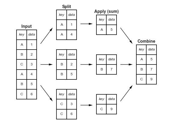
Group by: split-apply-combine

Functionality:

  • Grouping data by specific variables/column indices
  • Summarize/aggregate data by specific group features

How it works

“group by” is a common data wrangling process that exists in any language (R, Python, SQL) and refers to a process involving one or more of the following steps:

  • Splitting the data into groups based on some criteria.

  • Applying a function to each group independently.

  • Combining the results into a data structure.

From Python Data Science Handbook by Jake VanderPlas

groupby (it just splits!)

The groupby() method in pandas splits your dataset in smaller parts. It generates an iterable where each group is broken up into a tuple (group,data).

In [171]:
# load worldcup dataset
wc = pd.read_csv("WorldCups.csv")
wc_matches = pd.read_csv("WorldCupMatches.csv")

#groupby object
g = wc.groupby(["Winner"])
g
Out[171]:
<pandas.core.groupby.generic.DataFrameGroupBy object at 0x16c15a210>

The output of a groupby method is a flexible abstraction: although more complicated things are happening under the hood, in many ways, it can be treated as a collection of DataFrames. And as we learned, any collector can be iterated over!

In [172]:
# Iteration for groups
for group, data in g:
    print(group)
Argentina
Brazil
England
France
Germany
Germany FR
Italy
Spain
Uruguay
/var/folders/jy/10_nyhkn3nv_rrbnd8f_fr940000gp/T/ipykernel_52085/2794934486.py:2: FutureWarning: In a future version of pandas, a length 1 tuple will be returned when iterating over a groupby with a grouper equal to a list of length 1. Don't supply a list with a single grouper to avoid this warning.
  for group, data in g:
In [173]:
# iteration for data grouped
for group, data in g:
    print(data.head(2))
    Year    Country     Winner   Runners-Up   Third   Fourth  GoalsScored  \
10  1978  Argentina  Argentina  Netherlands  Brazil    Italy          102   
12  1986     Mexico  Argentina   Germany FR  France  Belgium          132   

    QualifiedTeams  MatchesPlayed Attendance  
10              16             38  1.545.791  
12              24             52  2.394.031  
   Year Country  Winner      Runners-Up   Third      Fourth  GoalsScored  \
5  1958  Sweden  Brazil          Sweden  France  Germany FR          126   
6  1962   Chile  Brazil  Czechoslovakia   Chile  Yugoslavia           89   

   QualifiedTeams  MatchesPlayed Attendance  
5              16             35    819.810  
6              16             32    893.172  
   Year  Country   Winner  Runners-Up     Third        Fourth  GoalsScored  \
7  1966  England  England  Germany FR  Portugal  Soviet Union           89   

   QualifiedTeams  MatchesPlayed Attendance  
7              16             32  1.563.135  
    Year Country  Winner Runners-Up    Third       Fourth  GoalsScored  \
15  1998  France  France     Brazil  Croatia  Netherlands          171   

    QualifiedTeams  MatchesPlayed Attendance  
15              32             64  2.785.100  
    Year Country   Winner Runners-Up        Third  Fourth  GoalsScored  \
19  2014  Brazil  Germany  Argentina  Netherlands  Brazil          171   

    QualifiedTeams  MatchesPlayed Attendance  
19              32             64  3.386.810  
   Year      Country      Winner   Runners-Up    Third   Fourth  GoalsScored  \
4  1954  Switzerland  Germany FR      Hungary  Austria  Uruguay          140   
9  1974      Germany  Germany FR  Netherlands   Poland   Brazil           97   

   QualifiedTeams  MatchesPlayed Attendance  
4              16             26    768.607  
9              16             38  1.865.753  
   Year Country Winner      Runners-Up    Third   Fourth  GoalsScored  \
1  1934   Italy  Italy  Czechoslovakia  Germany  Austria           70   
2  1938  France  Italy         Hungary   Brazil   Sweden           84   

   QualifiedTeams  MatchesPlayed Attendance  
1              16             17    363.000  
2              15             18    375.700  
    Year       Country Winner   Runners-Up    Third   Fourth  GoalsScored  \
18  2010  South Africa  Spain  Netherlands  Germany  Uruguay          145   

    QualifiedTeams  MatchesPlayed Attendance  
18              32             64  3.178.856  
   Year  Country   Winner Runners-Up   Third      Fourth  GoalsScored  \
0  1930  Uruguay  Uruguay  Argentina     USA  Yugoslavia           70   
3  1950   Brazil  Uruguay     Brazil  Sweden       Spain           88   

   QualifiedTeams  MatchesPlayed Attendance  
0              13             18    590.549  
3              13             22  1.045.246  
/var/folders/jy/10_nyhkn3nv_rrbnd8f_fr940000gp/T/ipykernel_52085/4250474981.py:2: FutureWarning: In a future version of pandas, a length 1 tuple will be returned when iterating over a groupby with a grouper equal to a list of length 1. Don't supply a list with a single grouper to avoid this warning.
  for group, data in g:

And we can acess a specific group:

In [73]:
g.get_group("Argentina")
Out[73]:
Year Country Winner Runners-Up Third Fourth GoalsScored QualifiedTeams MatchesPlayed Attendance
10 1978 Argentina Argentina Netherlands Brazil Italy 102 16 38 1.545.791
12 1986 Mexico Argentina Germany FR France Belgium 132 24 52 2.394.031

Aggreations (summarize)

The power of a grouping function (like .groupby() shines when coupled with an aggregation operation.

An aggregation is any operation that reduces the dimensionality of the data!

pandas: .groupby() + built-in methods

In [174]:
# mean of all numeric variables grouping by winners
wc.groupby(["Winner"]).mean()
/var/folders/jy/10_nyhkn3nv_rrbnd8f_fr940000gp/T/ipykernel_52085/2212436017.py:2: FutureWarning: The default value of numeric_only in DataFrameGroupBy.mean is deprecated. In a future version, numeric_only will default to False. Either specify numeric_only or select only columns which should be valid for the function.
  wc.groupby(["Winner"]).mean()
Out[174]:
Year GoalsScored QualifiedTeams MatchesPlayed
Winner
Argentina 1982.000000 117.000000 20.000000 45.000000
Brazil 1977.200000 122.400000 20.800000 43.000000
England 1966.000000 89.000000 16.000000 32.000000
France 1998.000000 171.000000 32.000000 64.000000
Germany 2014.000000 171.000000 32.000000 64.000000
Germany FR 1972.666667 117.333333 18.666667 38.666667
Italy 1965.000000 111.750000 21.750000 37.750000
Spain 2010.000000 145.000000 32.000000 64.000000
Uruguay 1940.000000 79.000000 13.000000 20.000000

or select a specific variable to perform the aggregation step on.

In [176]:
# With a specific input
wc.groupby(["Winner"])["GoalsScored"].mean()
Out[176]:
Winner
Argentina     117.000000
Brazil        122.400000
England        89.000000
France        171.000000
Germany       171.000000
Germany FR    117.333333
Italy         111.750000
Spain         145.000000
Uruguay        79.000000
Name: GoalsScored, dtype: float64

Notice the results come in a index structure. You can easily convert back to a fully formated dataframe by:

In [177]:
# reseting the index
wc.groupby(["Winner"])["GoalsScored"].mean().reset_index()
Out[177]:
Winner GoalsScored
0 Argentina 117.000000
1 Brazil 122.400000
2 England 89.000000
3 France 171.000000
4 Germany 171.000000
5 Germany FR 117.333333
6 Italy 111.750000
7 Spain 145.000000
8 Uruguay 79.000000
In [178]:
## as_index=false
wc.groupby(["Winner"], as_index=False)["GoalsScored"].mean()
Out[178]:
Winner GoalsScored
0 Argentina 117.000000
1 Brazil 122.400000
2 England 89.000000
3 France 171.000000
4 Germany 171.000000
5 Germany FR 117.333333
6 Italy 111.750000
7 Spain 145.000000
8 Uruguay 79.000000

Pandas offers many built-in methods to perform aggregations. Here is a list:

Built-in Methods

See user guide from Pandas Documentation

Method Functionality
.any Compute whether any of the values in the groups are truthy
.all Compute whether all of the values in the groups are truthy
.count Compute the number of non-NA values in the groups
.cov Compute the covariance of the groups
.first Compute the first occurring value in each group
.idxmax Compute the index of the maximum value in each group
.idxmin Compute the index of the minimum value in each group
.last Compute the last occurring value in each group
.max Compute the maximum value in each group
.mean Compute the mean of each group
.median Compute the median of each group
.min Compute the minimum value in each group
.nunique Compute the number of unique values in each group
.prod Compute the product of the values in each group
.quantile Compute a given quantile of the values in each group
.sem Compute the standard error of the mean of the values in each group
.size Compute the number of values in each group
.skew Compute the skew of the values in each group
.std Compute the standard deviation of the values in each group
.sum Compute the sum of the values in each group
.var Compute the variance of the values in each group

Let's see some examples:

In [179]:
# max goal by team as home team
(wc_matches
     .groupby(["Home Team Name"])
     ["Home Team Goals"]
     .max()
     .reset_index()
     .sort_values("Home Team Goals", ascending=False))
Out[179]:
Home Team Name Home Team Goals
31 Hungary 10
71 Yugoslavia 9
69 Uruguay 8
62 Sweden 8
25 Germany 8
... ... ...
56 Serbia 0
17 Czech Republic 0
64 Togo 0
32 IR Iran 0
77 rn">United Arab Emirates 0

78 rows × 2 columns

In [180]:
# number of matches as home team
(wc_matches
     .groupby(["Home Team Name"], as_index=False)
     ["Home Team Name"]
     .size()
     .sort_values("size", ascending=False)
)
Out[180]:
Home Team Name size
7 Brazil 82
35 Italy 57
2 Argentina 54
26 Germany FR 43
22 England 35
... ... ...
32 IR Iran 1
43 New Zealand 1
33 Iran 1
1 Angola 1
77 rn">United Arab Emirates 1

78 rows × 2 columns

pandas: .groupby() + agg()

Alternatively, we can specify a whole range of operations to aggregate by (along with specific variable columns) using the .aggregate()/.agg() method. To keep track of which operations correspond which variable, pandas will generate a hierarchical index for column entries.

In [181]:
wc.groupby(["Winner"])["GoalsScored"].agg(["mean","std","median"]).reset_index()
Out[181]:
Winner mean std median
0 Argentina 117.000000 21.213203 117.0
1 Brazil 122.400000 30.476220 126.0
2 England 89.000000 NaN 89.0
3 France 171.000000 NaN 171.0
4 Germany 171.000000 NaN 171.0
5 Germany FR 117.333333 21.594752 115.0
6 Italy 111.750000 40.532908 115.0
7 Spain 145.000000 NaN 145.0
8 Uruguay 79.000000 12.727922 79.0

We can also user-defined functions into the aggregate() function as well.

In [182]:
def mean_add_50(x):
    return np.mean(x) + 50

wc.groupby(["Winner"])["GoalsScored"].agg(["mean","std","median",mean_add_50])
Out[182]:
mean std median mean_add_50
Winner
Argentina 117.000000 21.213203 117.0 167.000000
Brazil 122.400000 30.476220 126.0 172.400000
England 89.000000 NaN 89.0 139.000000
France 171.000000 NaN 171.0 221.000000
Germany 171.000000 NaN 171.0 221.000000
Germany FR 117.333333 21.594752 115.0 167.333333
Italy 111.750000 40.532908 115.0 161.750000
Spain 145.000000 NaN 145.0 195.000000
Uruguay 79.000000 12.727922 79.0 129.000000

agg() + .rename() provides an easy workflow to rename your newly created variables

In [183]:
(wc.groupby(["Winner"])["GoalsScored"].
    agg(["mean","std","median",mean_add_50]).
    rename(columns={"mean": "goals_mean", 
                    "std": "goals_std",
                    "median": "goals_median", 
                    "mean_add_50":"mean_50_goals"})
)   
Out[183]:
goals_mean goals_std goals_median mean_50_goals
Winner
Argentina 117.000000 21.213203 117.0 167.000000
Brazil 122.400000 30.476220 126.0 172.400000
England 89.000000 NaN 89.0 139.000000
France 171.000000 NaN 171.0 221.000000
Germany 171.000000 NaN 171.0 221.000000
Germany FR 117.333333 21.594752 115.0 167.333333
Italy 111.750000 40.532908 115.0 161.750000
Spain 145.000000 NaN 145.0 195.000000
Uruguay 79.000000 12.727922 79.0 129.000000

pandas: .groupby() + .apply()

Even though I cover this in more details on the miscellaneous notebook, here is a good moment to bring the .apply() methods from pandas one more time.

The apply method lets you apply an arbitrary function by row or by columns on your data frame. As you can imagine, it also allow you to apply results by at a groupby object, and returns a summarizes dataset.

The function should take a DataFrame and returns either a Pandas object (e.g., DataFrame, Series) or a scalar

Let's an example with the mean add function:

In [184]:
(wc.groupby(["Country"])["GoalsScored"]. 
     apply(mean_add_50). 
     reset_index()
)
Out[184]:
Country GoalsScored
0 Argentina 152.0
1 Brazil 179.5
2 Chile 139.0
3 England 139.0
4 France 177.5
... ... ...
10 Spain 196.0
11 Sweden 176.0
12 Switzerland 190.0
13 USA 191.0
14 Uruguay 120.0

15 rows × 2 columns

multi-index grouping

We can also group by more than one variable (i.e. implement a multi-index on the rows).

In [185]:
wc.groupby(["Winner", "Year"])["GoalsScored"].mean().reset_index().head(5)
Out[185]:
Winner Year GoalsScored
0 Argentina 1978 102.0
1 Argentina 1986 132.0
2 Brazil 1958 126.0
3 Brazil 1962 89.0
4 Brazil 1970 95.0

pandas: .groupby() + .transform()

Other times we want to implement data manipulations by some grouping variable but retain structure of the original data. Put differently, our aim is not to aggregate but to perform some operation across specific groups.

To do so, we will combine .groupby() and .transform() methods. Let's see an example:

In [186]:
# create a new column
# notive you need to select the column you want to transform. 
wc.groupby(["Winner"])["GoalsScored"].transform("mean")
Out[186]:
0      79.000000
1     111.750000
2     111.750000
3      79.000000
4     117.333333
         ...    
15    171.000000
16    122.400000
17    111.750000
18    145.000000
19    171.000000
Name: GoalsScored, Length: 20, dtype: float64
In [188]:
# easily combined with assign
# create a new column
(wc.assign(goals_score_wc_mean_wc=wc.groupby(["Winner"])["GoalsScored"].
    transform("mean")))
Out[188]:
Year Country Winner Runners-Up Third Fourth GoalsScored QualifiedTeams MatchesPlayed Attendance goals_score_wc_mean_wc
0 1930 Uruguay Uruguay Argentina USA Yugoslavia 70 13 18 590.549 79.000000
1 1934 Italy Italy Czechoslovakia Germany Austria 70 16 17 363.000 111.750000
2 1938 France Italy Hungary Brazil Sweden 84 15 18 375.700 111.750000
3 1950 Brazil Uruguay Brazil Sweden Spain 88 13 22 1.045.246 79.000000
4 1954 Switzerland Germany FR Hungary Austria Uruguay 140 16 26 768.607 117.333333
... ... ... ... ... ... ... ... ... ... ... ...
15 1998 France France Brazil Croatia Netherlands 171 32 64 2.785.100 171.000000
16 2002 Korea/Japan Brazil Germany Turkey Korea Republic 161 32 64 2.705.197 122.400000
17 2006 Germany Italy France Germany Portugal 147 32 64 3.359.439 111.750000
18 2010 South Africa Spain Netherlands Germany Uruguay 145 32 64 3.178.856 145.000000
19 2014 Brazil Germany Argentina Netherlands Brazil 171 32 64 3.386.810 171.000000

20 rows × 11 columns

In [189]:
# also: very useful with lambda functions
wc.groupby("Winner")["GoalsScored"].transform(lambda x: x - x.mean())
Out[189]:
0     -9.000000
1    -41.750000
2    -27.750000
3      9.000000
4     22.666667
        ...    
15     0.000000
16    38.600000
17    35.250000
18     0.000000
19     0.000000
Name: GoalsScored, Length: 20, dtype: float64

Sorting values

In [190]:
# Pandas: sort values by a column variable (ascending)
wc.sort_values('Country').head(3)
Out[190]:
Year Country Winner Runners-Up Third Fourth GoalsScored QualifiedTeams MatchesPlayed Attendance
10 1978 Argentina Argentina Netherlands Brazil Italy 102 16 38 1.545.791
19 2014 Brazil Germany Argentina Netherlands Brazil 171 32 64 3.386.810
3 1950 Brazil Uruguay Brazil Sweden Spain 88 13 22 1.045.246
In [90]:
# Pandas: sort values by a column variable (descending)
wc.sort_values('Year',ascending=False).head(3)
Out[90]:
Year Country Winner Runners-Up Third Fourth GoalsScored QualifiedTeams MatchesPlayed Attendance
19 2014 Brazil Germany Argentina Netherlands Brazil 171 32 64 3.386.810
18 2010 South Africa Spain Netherlands Germany Uruguay 145 32 64 3.178.856
17 2006 Germany Italy France Germany Portugal 147 32 64 3.359.439
In [191]:
# Pandas: sort values by more than one column variable 
wc.sort_values(['Winner', "Country"]).head(3)
Out[191]:
Year Country Winner Runners-Up Third Fourth GoalsScored QualifiedTeams MatchesPlayed Attendance
10 1978 Argentina Argentina Netherlands Brazil Italy 102 16 38 1.545.791
12 1986 Mexico Argentina Germany FR France Belgium 132 24 52 2.394.031
6 1962 Chile Brazil Czechoslovakia Chile Yugoslavia 89 16 32 893.172

That was a lot! but you will get to keep this notebook for you!

And remember of the cheat sheet for pandas

Practice

Using the same ACLED data from the previous exercise, answer:

  1. What are the different event types recorded?

  2. How many events are recorded for each year?

  3. What’s the most common event type in the data?

  4. Which countries had the highest number of reported fatalities?

In [59]:
# 1
acled_sa = pd.read_csv("acled_south_america.csv")
acled_sa["event_type"].drop_duplicates().to_list()
Out[59]:
['Protests',
 'Battles',
 'Strategic developments',
 'Violence against civilians',
 'Riots',
 'Explosions/Remote violence']
In [60]:
# 2
(acled_sa.groupby("year", as_index=False)
     ["year"]
     .size()
        )       
Out[60]:
year size
0 2018 28758
1 2019 26441
2 2020 26615
3 2021 30190
4 2022 32039
5 2023 23544
In [61]:
# 3 
(acled_sa.groupby("event_type", as_index=False)
     ["event_type"]
     .size()
     .sort_values("size", ascending=False)
     .reset_index(drop=True)
        )    
Out[61]:
event_type size
0 Protests 80850
1 Battles 34042
2 Violence against civilians 30001
3 Riots 13447
4 Strategic developments 6917
5 Explosions/Remote violence 2330
In [62]:
acled_sa.groupby("country", as_index=False)["fatalities"].sum().sort_values("fatalities", ascending=False)
Out[62]:
country fatalities
2 Brazil 35842
4 Colombia 10553
13 Venezuela 8824
10 Peru 231
9 Paraguay 132
5 Ecuador 130
0 Argentina 117
3 Chile 108
1 Bolivia 88
11 Suriname 12
8 Guyana 11
12 Uruguay 7
7 French Guiana 2
6 Falkland Islands 0
In [ ]:
## Add your code here
In [101]:
!jupyter nbconvert _week-6c-data_wrangling_pandas.ipynb --to html --template classic
[NbConvertApp] Converting notebook _week-6c-data_wrangling_pandas.ipynb to html
[NbConvertApp] Writing 513144 bytes to _week-6c-data_wrangling_pandas.html