Introduction to Machine Learning
What is a Model?
- As social scientists, we are often interested in answering complex questions about human behavior. To answer them, we build models (theoretical and statistical).
A model is “a simplified representation of the reality created to serve a purpose.” (Provost & Fawcett 2013)
By definition:
Models are always a simplification of reality.
- We simplify so that we can understand and generalize a complex social process.
Models’ components come from assumptions we make about the world.
Models are all wrong, but some are useful.
An Statistical Model
The aim of statistical models is to estimate the relationship between the outcome and some set of variables:
\[ y = f(X) + \epsilon\]
Where:
\(y\) is the outcome/dependent/response variable
\(X\) is a matrix of predictors/features/independent variables
\(f()\) is some fixed but unknown function mapping X to y. The “signal” in the data
\(\epsilon\) is some random error term. The “noise” in the data
Statistical Learning
Statistical learning refers to a set of methods/approaches for estimating \(f(.)\)
\[ \hat{y} = \hat{f}(X)\]
Where \(\hat{f}(X)\) is an approximation of the “true” functional form, \(f(X)\)
\(\hat{y}\) is the predicted value of a true value y.
Inference (Social Science) vs Prediction (Machine Learning)
Two reasons we want to estimate \(f(\cdot)\):
\[ y_i = \beta_1*education_i + beta_2*gender_i + \sigma_i \]
Inference (Social Science) vs Prediction (Machine Learning)
Prediction
Goal is to predict values of the outcome, \(\hat{y}\)
\(\hat{f}(X)\) is treated as a black box
- model doesn’t need to be interpretable as long as it provides an accurate prediction of \(y\).
Key limitation:
- Interpretation: it is difficult to know which variables are doing the heavy lifting and the exact influence of \(x\) on \(y\).
Example: giving a k number of features, and all possible interactions between them,how likely is each voter i to turnout?
This is the machine learning tradition/predictive modeling/AI
Reducible vs. Irreducible Error
- When we build models, the aim is to find a \(\hat{f}(X)\) that minimizes the error in the model.
\[\text{total error} = E(y - \hat{y})^2\] \[ = E[f(X) + \epsilon - \hat{f}(X) ]^2\]
\[= \underbrace{E[f(X) -\hat{f}(X)]^2}_{\text{Reducible}} + \underbrace{var(\epsilon)}_{\text{Irreducible}}\]
The “reducible” error is the systematic signal. We can reduce this error by using different functional forms, better data, or a mixture of those two.
The “irreducible” error is associated with the random noise around \(y\).
Statistical learning is concerned with minimizing the reducible error.
Our predictions will never be perfect given the irreducible error.
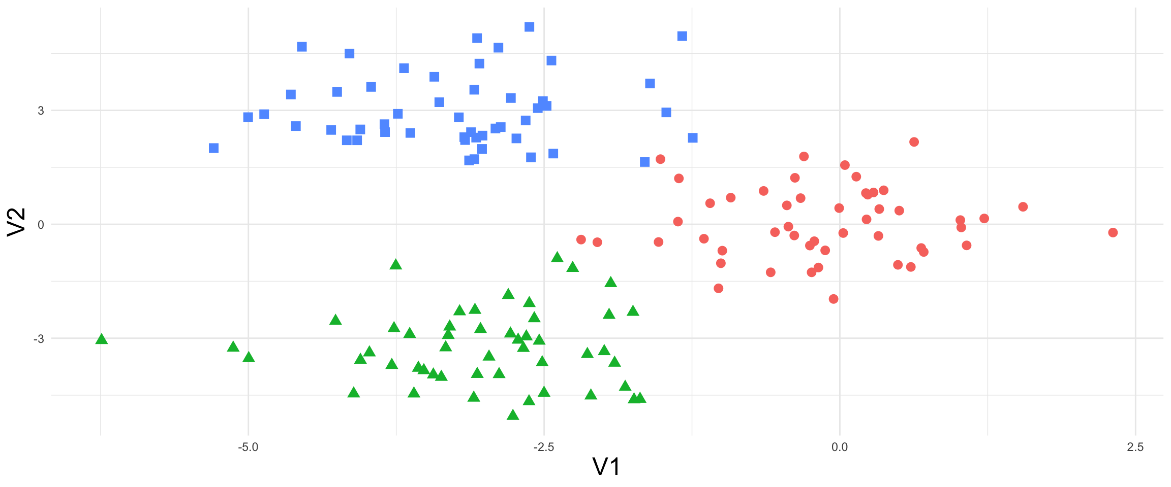
Supervised and Unsupervised Machine Learning
Supervised and Unsupervised Learning
Types of Models
![]()
Machine Learning: what does learning mean?
For inferential work (in your stats class), you get some data, and you estimate a model using the entire data. This is not what we do in machine learning.
A Machine Learning Pipeline
The purpose of training the model is to capture signal and ignore noise.
To do so:
Define a accuracy metric:
- In the regression setting, the most common accuracy metric is mean squared error (MSE).
- Mean Squared Error = \(\frac{\sum^N_{i=1} (y_i - \hat{f}(X_i))^2}{N}\)
Train-Test Split
Split your data between training and test
Training data: find the best model and tune the parameters of these models
Test data: assess the accuracy of your model.
Select the model based on smaller out of sample predictive accuracy, using UNSEEN data.
Workflow: Inference vs ML
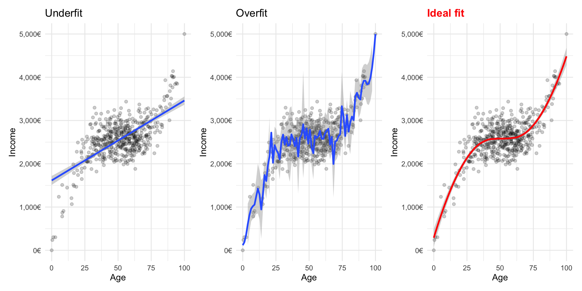
What can go wrong? Bias and Variance Trade-off
Expected prediction error for a data point:
\[
E\big[(\hat{y} - y)^2\big] = (E[\hat{f}(x)] - f(x))^2 + E\Big[\big(\hat{f}(x) - E[\hat{f}(x)]\big)^2\Big] + \epsilon
\]
Bias: Difference between the expected prediction of the model and the true value.
\[\text{Bias}(\hat{f}(x)) = E[\hat{f}(x)] - f(x)\]
Variance: How much do the model’s predictions fluctuate for different training sets?
\[
\text{Var}(\hat{f}(x)) = E\Big[\big(\hat{f}(x) - E[\hat{f}(x)]\big)^2\Big]
\]
Bias and Variance Tradeoff:
Bias and Variance Trade-off
![]()
- Trade-off: as we reduce bias, we risk overfiting. Training properly is key to find a middle-of-the-road solution.
Challenge: avoid overfitting the data
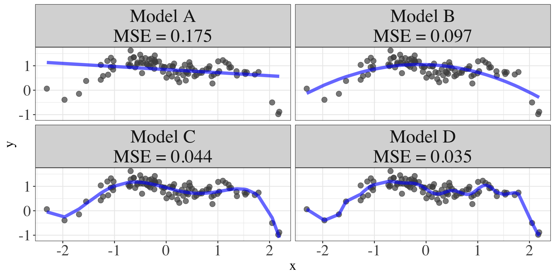
![]()
MSE Training Data
![]()
Quizz:
- Which model will perform worse if we are to throw some unseen data?
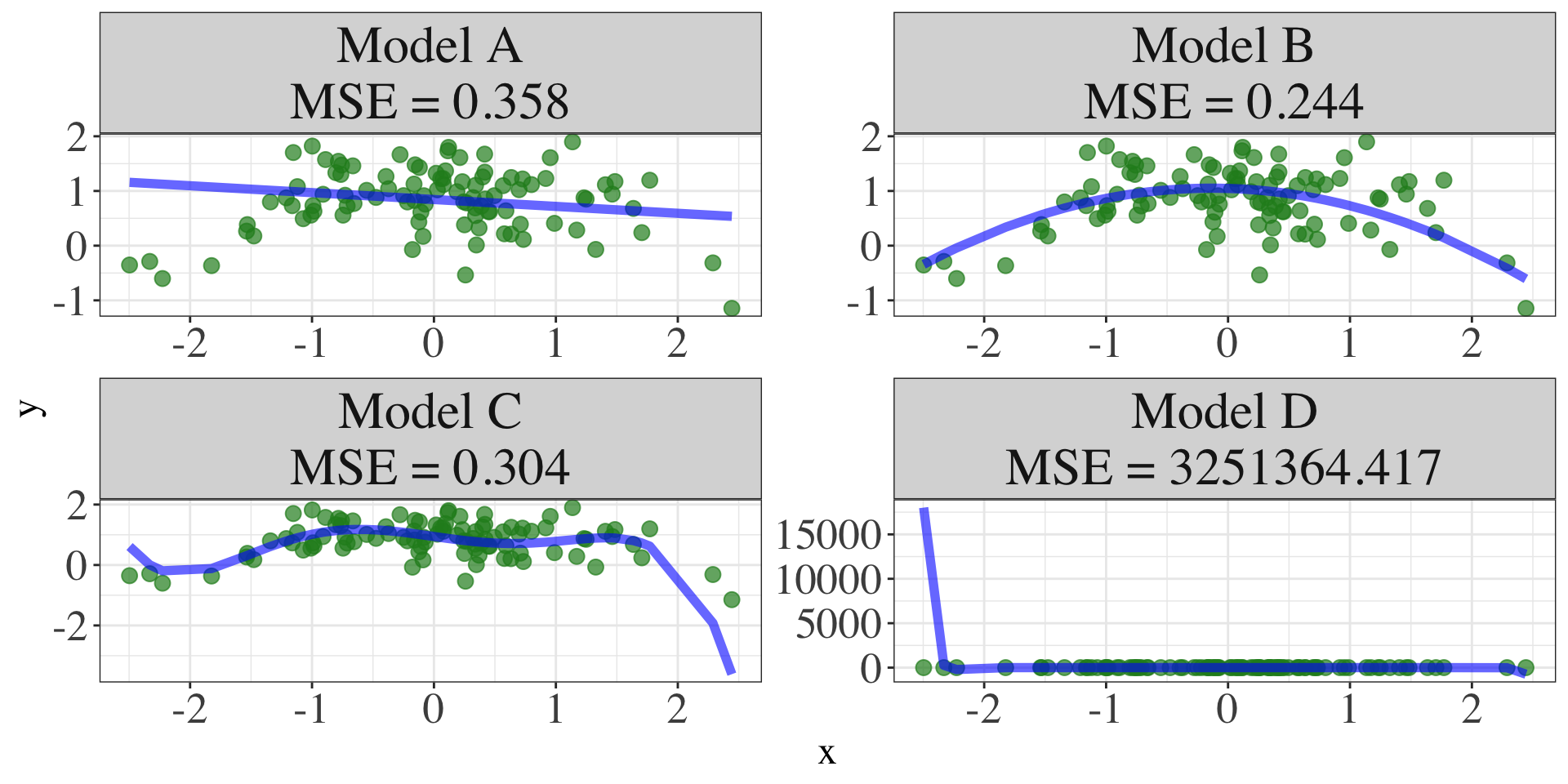
Model Accuracy: Out-Sample Prediction
![]()
Train-Validation-Test
Training Set
- Largest portion (60-80% of the data)
- To train the model
Validation Set
- Smaller portion (10-20% of data)
- Check different models
- To tune hyperparameters and evaluate model during training
- Parameters that we set before training begins (e.g. learning rate, number of neural networks layers, strength of regularization)
Test Set - Smaller portion (10-20% of data) - To assess final model performance
Training the Model: Cross-Validation
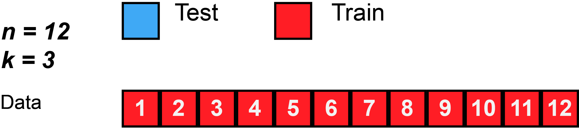
K-Fold Cross Validation
K-Fold Cross Validation involves randomly dividing the data into \(k\) groups (or folds). Model is trained on \(k-1\) folds, then test on the remaining fold.
Process is repeated \(k\) times, each time using a new fold.
Offers \(k\) estimates of the test error, which we average to calculate the error
Quizz:
What is the difference between inferential models vs predictive modelling? In which one do you care about unbiased estimators?
Can I use an OLS model for a predictive task? If so, will an OLS model show lean torward high bias and low variance or low bias and high variance?
What happens if I make decisions about which model to fit by ALWAYS looking at the error in the test set?