PPOL 5203 - Data Science I: Foundations

Week 10: Text-As-Data I: Description and Topics

Professor: Tiago Ventura

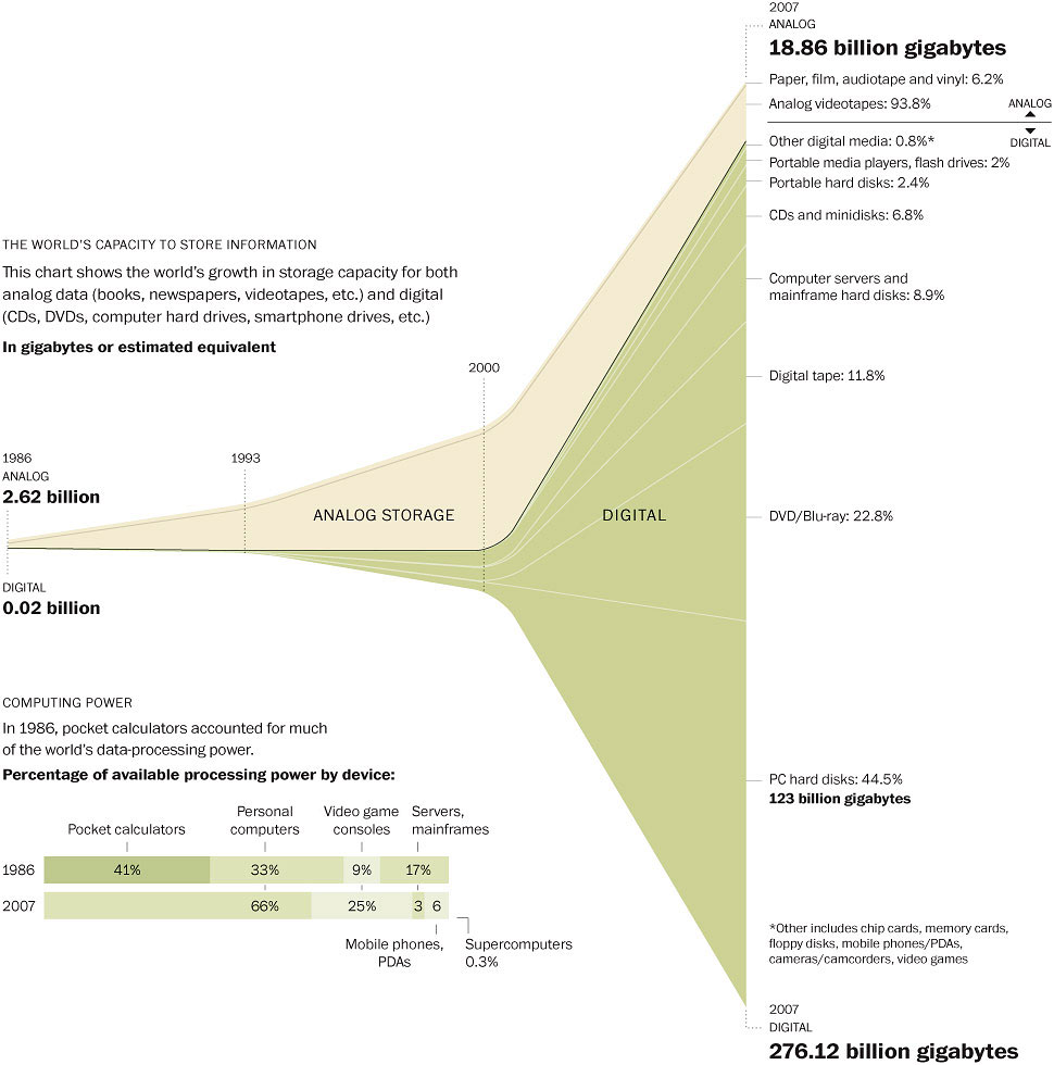
A significant part of how we produce and store data is textual

Modeling Text as Data

Why do we need models to analyze text data?

Scalability and Dimensionality Reduction

• Humans are great at understanding the meaning of a sentence or a document in-depth

• Computers are better at understanding patterns, classify and describe content across millions of subjects

• Computational Text analysis augments humans – does not replace us

• Statistical models + Powerful Computers allows us to process data at scale and understand common patterns

• We know “All text models are wrong” – This is particularly true with text!

Workflow

• Acquire textual data:

  • Existing corpora; scraped data; digitized text

• Preprocess the data:

  • Bag-of-words
  • Reduce noise, capture signal

Workflow

• Apply method appropriate to research goal:

  • Descriptive Analysis:
    • Count Words, Readability; similarity;
  • Classify documents into unknown categories
    • Document clustering
    • Topic models
  • Classify documents into known categories
    • Dictionary methods
    • Supervised machine learning
    • Transfer-Learning - use models trained in text for other purposes

Already did it!

• Acquire textual data:
  • Existing corpora; scraped data; digitized text

Today:

• Preprocess the data:

  • Convert text to numbers.
  • Use the Bag-of-words assumption.
  • Reduce noise, capture signal

• Apply methods appropriate to research goal:

  • Descriptive Analysis:
    • Count Words, Readability; similarity;
  • Classify documents into unknown categories
    • Topic models

Next Week:

• Classify documents into known categories
  • Dictionary methods
  • Supervised machine learning
  • Transfer-Learning - use models trained in text for other purposes

Very quick introdution! Want learn more? Take the Text-as-Data Class in the future.

From Text-to-Numbers: Representing Texts as Data.

When working with text, we have two critical challenges:

• Reduce Textual Complexity (Think about every word as a variable. This is huge matrix!!)

  • Pre-Processing steps

• Convert unstructured text to numbers ~ that we can feed in to a statistical model

  • Document Feature Matrix/Bag-of-Words

Reducing Complexity: Pre-Processing Steps

• Tokenize: break out larger chunks of text in words (unigram) or n-grams

• Lowercase: convert all to lower case

• Remove Noise: stopwords, numbers, punctuation, function words

• Stemming: chops off the ends of words

• Lemmatization: doing things properly with the use of a vocabulary and morphological analysis of words

Example

Text

We use a new dataset containing nearly 50 million historical newspaper pages from 2,700 local US newspapers over the years 1877–1977. We define and discuss a measure of power we develop based on observed word frequencies, and we validate it through a series of analyses. Overall, we find that the relative coverage of political actors and of political offices is a strong indicator of political power for the cases we study

After pre-processing

use new dataset contain near 50 million historical newspaper pag 2700 local u newspaper year 18771977 define discus measure power develop bas observ word frequenc validate ser analys overall find relat coverage political actor political offic strong indicator political power cas study

Text Representation

• Represent text as an unordered set of tokens in a document. Bag-of-Words Assumption

• While order is ignored, frequency matters!

• To represent documents as numbers, we will use the vector space model representation:

  • A document \(D_i\) is represented as a collection of features \(W\) (words, tokens, n-grams..)

  • Each feature \(w_i\) can be placed in a real line, then a document \(D_i\) is a vector with \(W\) dimensions

Imagine the sentence below: “If that is a joke, I love it. If not, can’t wait to unpack that with you later.”

• Sorted Vocabulary =(a, can’t, i, if, is, it, joke, later, love, not, that, to, unpack, wait, with, you”)

• Feature Representation = (1, 1, 1, 2, 1, 1, 1, 1, 1, 1, 2, 1, 1, 1, 1, 1)

• Features will typically be the n-gram (mostly unigram) frequencies of the tokens in the document, or some function of those frequencies

Each document becomes a numerical vector (vector space model)

• stacking these vectors will give you our workhose representation for text: Document Feature Matrix

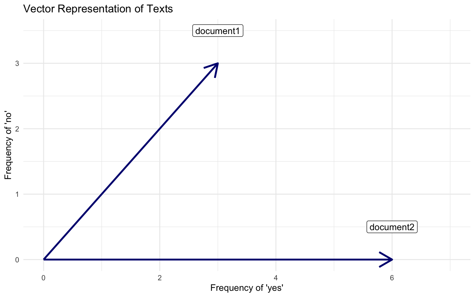
Visualizing Vector Space Model

Documents

Document 1 = “yes yes yes no no no”

Document 2 = “yes yes yes yes yes yes”

From Text to Numbers: Bag-of-Words & Document-Feature Matrix

Text-as-Data methods today

• Comparing/Describing Documents

• Topic Models: Finding hidden structures in a corpus

Comparing Documents: How `far’ is document a from document b?

Using the vector space, we can use notions of geometry to build well-defined comparison/similarity measures between the documents.

• in multiple dimensions!!

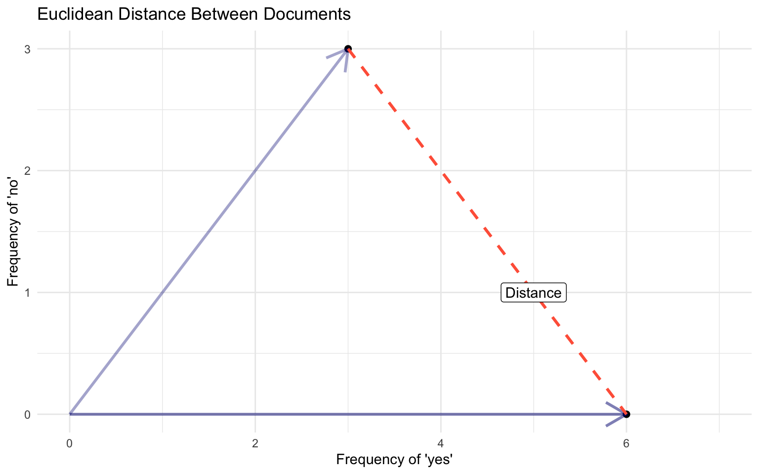
Euclidean Distance

The ordinary, straight line distance between two points in space. Using document vectors \(y_a\) and \(y_b\) with \(j\) dimensions

Euclidean Distance

\[ ||y_a - y_b|| = \sqrt{\sum^{j}(y_{aj} - y_{bj})^2} \]

Can be performed for any number of features J ~ has nice mathematical properties

no negative distances: sij   0 2 distance between documents is zero () documents are identical 3 distance between documents is symmetric: sij = sji 4 measures satisfy triangle inequality. sik   sij + sjk

Euclidean Distance, example

Euclidean Distance

\[ ||y_a - y_b|| = \sqrt{\sum^{j}(y_{aj} - y_{bj})^2} \]

• \(y_a\) = [0, 2.51, 3.6, 0] and \(y_b\) = [0, 2.3, 3.1, 9.2]

• \(\sum_{j=1}^j (y_a - y_b)^2\) = \((0-0)^2 + (2.51-2.3)^2 + (3.6-3.1)^2 + (9-0)^2\) = \(84.9341\)

• \(\sqrt{\sum_{j=1}^j (y_a - y_b)^2}\) = 9.21

Exercise

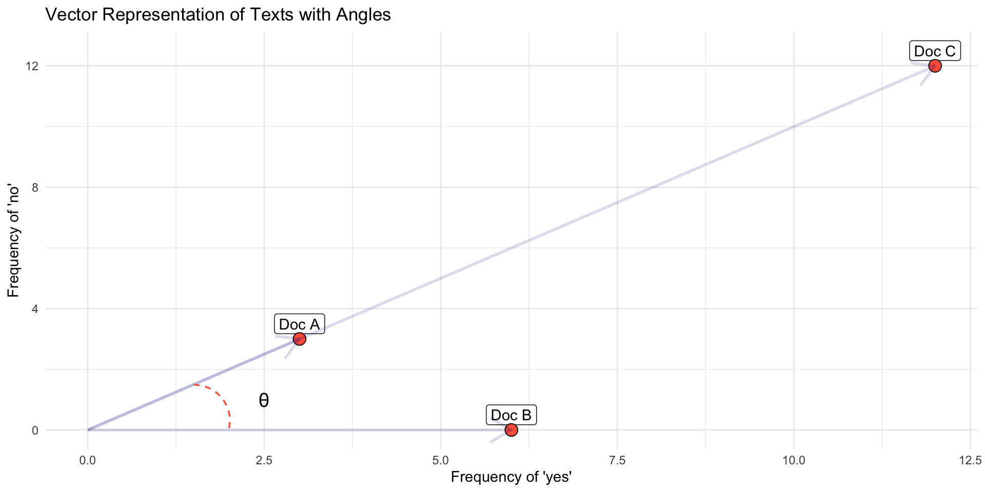
Documents, W=3 {yes, no}

Document 1 = “yes yes yes no no no” (3, 3)

Document 2 = “yes yes yes yes yes yes” (6,0)

Document 3= “yes yes yes no no no yes yes yes no no no yes yes yes no no no yes yes yes no no no” (12, 12)

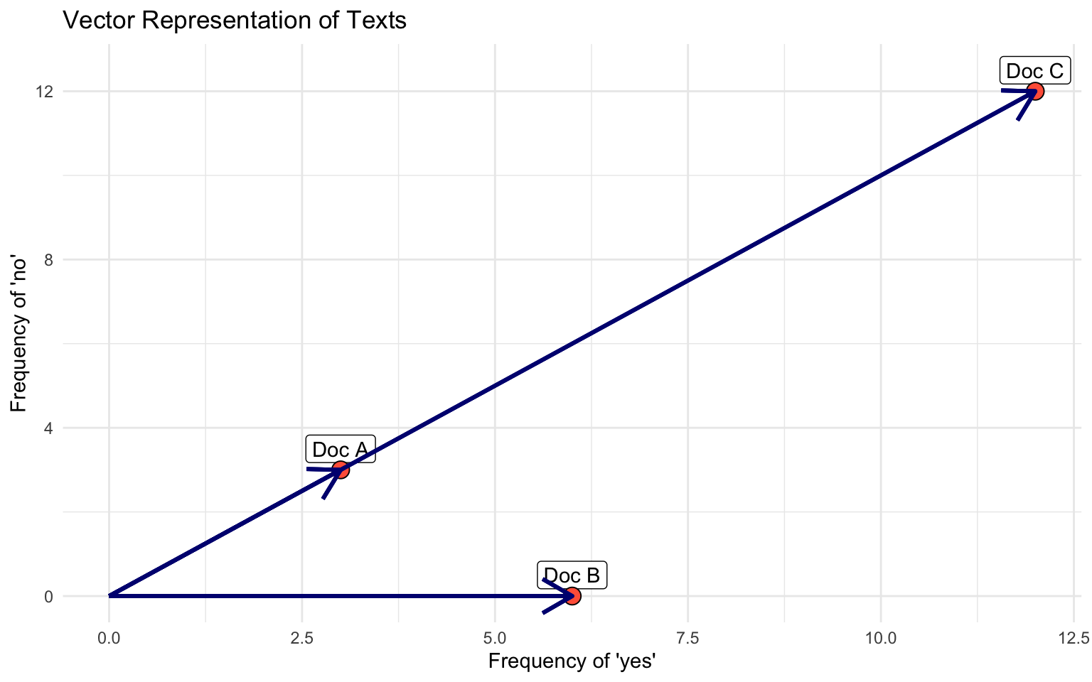
• Which documents will the euclidean distance place closer together?
• Does it look like a good measure for similarity?
  • Doc C = Doc A * 3

Cosine Similarity

Euclidean distance rewards magnitude, rather than direction

\[ \text{cosine similarity}(\mathbf{y_a}, \mathbf{y_b}) = \frac{\mathbf{y_a} \cdot \mathbf{y_b}}{\|\mathbf{y_a}\| \|\mathbf{y_b}\|} \]

• \(U \cdot V\) ~ dot product between vectors

  • it is a projection of one vector into another
  • Works as a measure of similarity
  • But rewards magnitude

• \(||\mathbf{U}||\) ~ vector magnitude, length ~ \(\sqrt{\sum{u_{i}^2}}\)

  • normalizes a vector projection of documents’ by their lengths

• cosine similarity captures some notion of relative direction controlling for different magnitudes.

Cosine Similarity

Cosine function has a range between -1 and 1.

• Consider: cos (0) = 1, cos (90) = 0, cos (180) = -1

Topic Models: LDA Approach

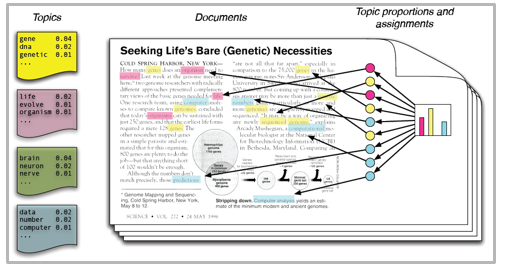
Topic Models: Intuition

• Problem: Once we start with docs, we do not know what topics exist, what words belong to which topics, what topic proportions each document has

• Probabilistic Model: Make assumptions about how language work, and how topics emerge. Then check if this matches with word co-occurrence in each document

• Documents: formed from probability distribution of topics

  • a speech can be 40% about trade, 30% about sports, 10% about health, and 20% spread across topics you don’t think make much sense

• Topics: formed from probability distribution over words

  • the topic health will have words like hospital, clinic, dr., sick, cancer

Blei, 2012,

Intuition: Language Model

• Step 1: For each document:

  • Randomly choose a distribution over topics. That is, choose one of many multinomial distributions, each which mixes the topics in different proportions.

• Step 2: For each topic

  • Randomly choose a distribution of words, also from one of many multinomial distributions., each with mixes words in different proportions

• Step 3: Then, for every word in the document

  • Randomly choose a topic from the distribution over topics from step 1.
  • Randomly choose a word from the distribution over the vocabulary that the topic implies.

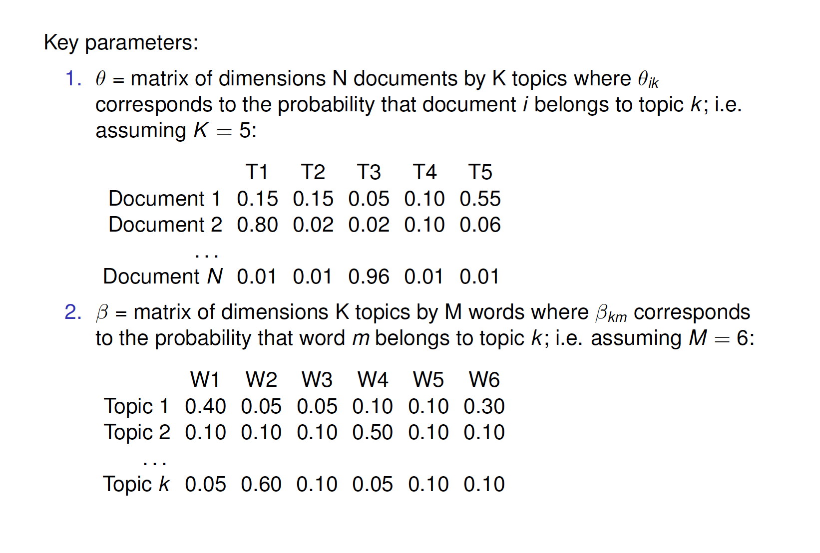
Inference: How to estimate all these parameters?

Inference: Use the observed data, the words, to make an inference about the latent parameters: the \(\beta\)s, and the \(\theta\)s.

Complicate Math: Using the observed data, the words, we can estimate latent parameters. We start with the joint distribution implied by our language model (Blei, 2012):

\[ p(\beta_{1:K}, \theta_{1:D}, z_{1:D}, w_{1:D})= \prod_{K}^{i=1}p(\beta_i)\prod_{D}^{d=1}p(\theta_d)(\prod_{N}^{n=1}p(z_{d,n}|\theta_d)p(w_{d,n}|\beta_{1:K},z_{d,n}) \]

To get to this conditional:

\[ p(\beta_{1:K}, \theta_{1:D}, z_{1:D}|w_{1:D})=\frac{p(\beta_{1:K}, \theta_{1:D}, z_{1:D}, w_{1:D})}{p(w_{1:D})} \]

Estimation: Use Gibbs Sampling (Bayesian Stats) to reverse-engineer this

• Start at random for all parameters, compare with word co-occurrence within docs, and update

• Why it works: The model wants a topic to contain as few words as possible, but a document to contain as few topics as possible. This tension is what makes the model work.

Show me results!

Many different types of topic models

• Structural topic model: allow (1) topic prevalence, (2) topic content to vary as a function of document-level covariates (e.g., how do topics vary over time or documents produced in 1990 talk about something differently than documents produced in 2020?); implemented in stm in R (Roberts, Stewart, Tingley, Benoit)

• Correlated topic model: way to explore between-topic relationships (Blei and Lafferty, 2017); implemented in topicmodels in R; possibly somewhere in Python as well!

• Keyword-assisted topic model: seed topic model with keywords to try to increase the face validity of topics to what you’re trying to measure; implemented in keyATM in R (Eshima, Imai, Sasaki, 2019)

• BertTopic: BERTopic is a topic modeling technique that leverages transformers and TF-IDF to create dense clusters of words.

Notebooks