Tidyverse II: Tidyr and Stringr

class: center, middle, inverse, title-slide

# Tidyverse II: Tidyr and Stringr
## IPSA-Flacso Summer School
### Tiago Ventura

---

# Introduction

Yesterday, we had our first immersion in using tidyverse for data manipulation.

Today we will take a few new steps.

You will learn two new skills/packages:

- Tidy your data, with `tidyr`

- Manipulate strings, with `stringr`

---
class:inverse, middle, center

# Tidy Data.

---

## Tidy Data

#### [Wickham, H. (2014). Tidy data. Journal of statistical software, 59(10), 1-23.](https://vita.had.co.nz/papers/tidy-data.pdf)

The `tidyverse` framework comes from the concept of `tidy` data. Which means that all the packages on `tidyverse` work at full-speed when combined with a dataset organized in the tidy format.

A `tidy` data is just an specific way to organize your data. You can organize on different ways, but I will try to convice you about being consistent and having the tidy format as your baseline.

There are three interrelated rules which make a [dataset tidy](https://r4ds.had.co.nz/tidy-data.html).

- Each variable must have its own column.
- Each observation must have its own row.
- Each value must have its own cell.

---

# Visually

![](./figs/tidy-1.png)

---
# Advantages

These three simple definitions have several advantages:

- It gives you a consistent way to organize our databases.

- Saving one variable per column facilitates manipulation operations (R works better with column vectors).

- Integrates with other `tidyverse` packages.

---

## Tidy Data: Gapminder

```r
library(gapminder)
gapminder 
```

```
## # A tibble: 1,704 x 6
##    country     continent  year lifeExp      pop gdpPercap
##    <fct>       <fct>     <int>   <dbl>    <int>     <dbl>
##  1 Afghanistan Asia       1952    28.8  8425333      779.
##  2 Afghanistan Asia       1957    30.3  9240934      821.
##  3 Afghanistan Asia       1962    32.0 10267083      853.
##  4 Afghanistan Asia       1967    34.0 11537966      836.
##  5 Afghanistan Asia       1972    36.1 13079460      740.
##  6 Afghanistan Asia       1977    38.4 14880372      786.
##  7 Afghanistan Asia       1982    39.9 12881816      978.
##  8 Afghanistan Asia       1987    40.8 13867957      852.
##  9 Afghanistan Asia       1992    41.7 16317921      649.
## 10 Afghanistan Asia       1997    41.8 22227415      635.
## # … with 1,694 more rows
```

---

## Tidy vs Untidy

---

## Untidy: Wide Data.

Untidy data are usually referred as wide data. Some of your have already heard this term, I am sure.

```r
wide <- tibble(pais=c("Brasil", "Uruguai", "Chile"), 
               pres_ano_2010= c("Lula", "Mujica", "Pinera"), 
               pres_ano_2014=c("Dilma", "Tabare", "Bachelet"), 
               pres_ano_2018=c("Temer", "Lacalle", "Pinera"))
wide
```

```
## # A tibble: 3 x 4
##   pais    pres_ano_2010 pres_ano_2014 pres_ano_2018
##   <chr>   <chr>         <chr>         <chr>        
## 1 Brasil  Lula          Dilma         Temer        
## 2 Uruguai Mujica        Tabare        Lacalle      
## 3 Chile   Pinera        Bachelet      Pinera
```

---

## Challenge

### Tidy or Untidy ?

```r
tab <- tibble(pais=c("Brasil", "Uruguai", "Argentina"),
       i_2010 = c(5, 1, 2), 
       i_2014 = c(10, 9, 9),
       i_2018 = c(0, 1, 2))
tab 
```

```
## # A tibble: 3 x 4
##   pais      i_2010 i_2014 i_2018
##   <chr>      <dbl>  <dbl>  <dbl>
## 1 Brasil         5     10      0
## 2 Uruguai        1      9      1
## 3 Argentina      2      9      2
```

---

### Tidy or Untidy ?

```r
tab1 <- tibble(pais=c("Brasil", "Argentina"),
       ano = c(2020, 2020),
       presidente_vice = c("Bolsonaro-Mourão", "Fernandez-Kirchner"))

tab1 
```

```
## # A tibble: 2 x 3
##   pais        ano presidente_vice   
##   <chr>     <dbl> <chr>             
## 1 Brasil     2020 Bolsonaro-Mourão  
## 2 Argentina  2020 Fernandez-Kirchner
```

---

### Tidy or Untidy ?

```r
tab2 <- tibble(pais=c("Brasil", "Brasil",  "Argentina", "Argentina"),
       ano = c(2020, 2020, 2020, 2020), 
       covid = c("Casos", "Vacinas", "Casos", "Vacinas"), 
       numero= c(10500000, 6535363, 2100000, 1800000))
tab2
```

```
## # A tibble: 4 x 4
##   pais        ano covid     numero
##   <chr>     <dbl> <chr>      <dbl>
## 1 Brasil     2020 Casos   10500000
## 2 Brasil     2020 Vacinas  6535363
## 3 Argentina  2020 Casos    2100000
## 4 Argentina  2020 Vacinas  1800000
```

---

# tidyr

We will use the functions from the `tidyr` package to move between tidy<->untidy data.

Four main functions:

- `pivot_longer()`

- `pivot_wider()`

- `separate()`

- `unite()`

---

## pivot_longer

#### Multiple columns -> A single columns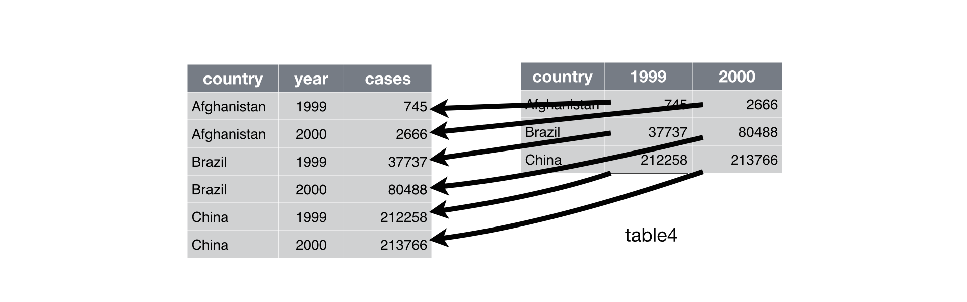

![](./figs/gather.png)

---

`pivot_longer()` has Three main inputs:

- `cols`: columns to pivot into longer format
- `names_to`: A string specifying the **name** of the column to stores the **name* of the old columns.
- `values_to`: A string specifying the **name** of the column to stores the **name* of the old columns.

---

## Exampe

```r
# Before = Wide 
wide
```

```r
# Pivoting

wide %>%
  pivot_longer(cols=c(pres_ano_2010, pres_ano_2014, 
                      pres_ano_2018), 
               names_to="presidente_ano", 
               values_to="presidente")
```

```
## # A tibble: 9 x 3
##   pais    presidente_ano presidente
##   <chr>   <chr>          <chr>     
## 1 Brasil  pres_ano_2010  Lula      
## 2 Brasil  pres_ano_2014  Dilma     
## 3 Brasil  pres_ano_2018  Temer     
## 4 Uruguai pres_ano_2010  Mujica    
## 5 Uruguai pres_ano_2014  Tabare    
## 6 Uruguai pres_ano_2018  Lacalle   
## 7 Chile   pres_ano_2010  Pinera    
## 8 Chile   pres_ano_2014  Bachelet  
## 9 Chile   pres_ano_2018  Pinera
```

---

### Another Example:

```r
tab %>%
  pivot_longer(cols = c(starts_with("i")), 
               names_to="t", 
               values_to="values")
```

```
## # A tibble: 9 x 3
##   pais      t      values
##   <chr>     <chr>   <dbl>
## 1 Brasil    i_2010      5
## 2 Brasil    i_2014     10
## 3 Brasil    i_2018      0
## 4 Uruguai   i_2010      1
## 5 Uruguai   i_2014      9
## 6 Uruguai   i_2018      1
## 7 Argentina i_2010      2
## 8 Argentina i_2014      9
## 9 Argentina i_2018      2
```

---

## pivot_wider

### (Openning one column -> Several)

---

### Basics

`pivote_wider()` has two main inputs

- `names_from`: name of the column with names to be opened.
- `values_from`: name of the columns with values to be opened.

---

## Example

```r
tab2
```

```r
# untidying
tab2 %>%
  pivot_wider(names_from=covid, 
              values_from=numero)
```

```
## # A tibble: 2 x 4
##   pais        ano    Casos Vacinas
##   <chr>     <dbl>    <dbl>   <dbl>
## 1 Brasil     2020 10500000 6535363
## 2 Argentina  2020  2100000 1800000
```
---

## Example II: Filling NAs

```r
tab2 <- tab2 %>%
        add_row(pais="Uruguai", 
                ano=2020, 
                covid="Casos", 
                numero=8919)
```

.pull-left[

### With Missings.

```r
# tidying with Missings
tab2 %>%
  pivot_wider(names_from=covid, 
              values_from=numero)
```

```
## # A tibble: 3 x 4
##   pais        ano    Casos Vacinas
##   <chr>     <dbl>    <dbl>   <dbl>
## 1 Brasil     2020 10500000 6535363
## 2 Argentina  2020  2100000 1800000
## 3 Uruguai    2020     8919      NA
```

]

--
.pull-right[

### Filling the Missings.

```r
# tidying Com Missings
tab2 %>%
  pivot_wider(names_from=covid, 
              values_from=numero, 
*             values_fill=0)
```

```
## # A tibble: 3 x 4
##   pais        ano    Casos Vacinas
##   <chr>     <dbl>    <dbl>   <dbl>
## 1 Brasil     2020 10500000 6535363
## 2 Argentina  2020  2100000 1800000
## 3 Uruguai    2020     8919       0
```

]
--

---
## Separate and Unite

Two last functions to conclude: `separate()` e `unite()`.

- `separate()`: Separate a character column into multiple columns with a regular expression

- `unite()`: Unite multiple columns into one

```r
tab1 %>%
  separate(presidente_vice, into=c("presidente", "vice"), 
                            sep="-")
```

```
## # A tibble: 2 x 4
##   pais        ano presidente vice    
##   <chr>     <dbl> <chr>      <chr>   
## 1 Brasil     2020 Bolsonaro  Mourão  
## 2 Argentina  2020 Fernandez  Kirchner
```

---
class: middle, center, inverse

## Manipulating Strings

---

## Strings

Strings = character variables.

We will learn several functions to manipulate strings in R. Fundamental for our future classes on scrapping and text analysis.

Those functions are from the package `stringr`. And the package follows the `tidyverse` logic.

We will also conclude with an intro to regular expressions.

---
## stringr

The `stringr`, as all the other packages on tidyverse, is a verb-based package. This means that the name of the function intuitively explain its usage.

`stringr` functions have two components:

- all the functions start with `str`

- followed by the verb-based component ~> `str_remove` to remove some textual pattern.

See a complete list of the stringr functions [here](https://evoldyn.gitlab.io/evomics-2018/ref-sheets/R_strings.pdf)

---
## Detect Textual Patterns

Two components:

- First Argument: textual input

- Second Argument: textual pattern to be detected

---

`str_detect()`

```r
str_detect(c("Tiago", "Ventura"), "Ventura")
```

```
## [1] FALSE  TRUE
```

`str_count()`

```r
str_count(c("Tiago", "Ventura"), "Ventura")
```

```
## [1] 0 1
```

---

`str_locate()`

```r
str_locate(c("Tiago#umd", "Ventura#fgv"), "#")
```

```
##      start end
## [1,]     6   6
## [2,]     8   8
```

---
## Functions to Change Strings.

`str_replace_all()`

```r
str_replace_all(c("Tiago#umd", "Ventura#fgv"), "#", " ")
```

```
## [1] "Tiago umd"   "Ventura fgv"
```

`str_to_lower()`

```r
str_to_lower(c("Tiago#umd", "Ventura#fgv"))
```

```
## [1] "tiago#umd"   "ventura#fgv"
```

---
## Working with dataframes

As a package from `tidyverse`, the `stringr` functions were designs to work perfectly with dataframes/tibbles.

### Downloading Candidates Data in Brazil.

Let's see some examples using an set political candidates' names from Brazil Legislative Elections.

```r
cand <- get_candidates(year=2018,
                       position="Federal Deputy") %>%
          as_tibble()
```

---

## Stringr + Mutate

Easy to create new variables.

```r
cand %>%
  select(NOME_URNA_CANDIDATO) %>%
  mutate(nome_minusculo=str_to_lower(NOME_URNA_CANDIDATO))
```

```
## # A tibble: 8,588 x 2
##    NOME_URNA_CANDIDATO    nome_minusculo        
##    <chr>                  <chr>                 
##  1 "PASTOR MANUEL MARCOS" "pastor manuel marcos"
##  2 "JUNIOR PARIS DAKAR"   "junior paris dakar"  
##  3 "RUDILEI ESTRELA"      "rudilei estrela"     
##  4 "NELSON SALES"         "nelson sales"        
##  5 "EURICO CORDEIRO "     "eurico cordeiro "    
##  6 "DJÊ CAVALCANTE"       "djê cavalcante"      
##  7 "PAULO SORIANO"        "paulo soriano"       
##  8 "JESUS SÉRGIO"         "jesus sérgio"        
##  9 "CHICO DOIDO DA SAÚDE" "chico doido da saúde"
## 10 "CABRAL"               "cabral"              
## # … with 8,578 more rows
```

---

## Extract Textual Patterns

Two main components

- First Argument: textual input

- Second Argument: Textual pattern.

```r
# Lets transform this collumn to a vector just os show a few more easy examples

nomes<-cand$NOME_URNA_CANDIDATO[1:10]
```

---

`str_sub()`: extract by position

```r
str_sub(nomes, 1, 5)
```

```
##  [1] "PASTO" "JUNIO" "RUDIL" "NELSO" "EURIC" "DJÊ C" "PAULO" "JESUS" "CHICO"
## [10] "CABRA"
```

`str_subset()`: extract with a pattern

```r
str_subset(nomes, "PASTOR")
```

```
## [1] "PASTOR MANUEL MARCOS"
```

---

`str_extract_all()`: extract only the pattern.

```r
str_extract_all(nomes, "PASTOR|CHICO") # | = or
```

```
## [[1]]
## [1] "PASTOR"
## 
## [[2]]
## character(0)
## 
## [[3]]
## character(0)
## 
## [[4]]
## character(0)
## 
## [[5]]
## character(0)
## 
## [[6]]
## character(0)
## 
## [[7]]
## character(0)
## 
## [[8]]
## character(0)
## 
## [[9]]
## [1] "CHICO"
## 
## [[10]]
## character(0)
```

]

---

## How to write more general patterns?

Quite often we look for more general patterns in our textual searches. For example:

- All sentences that end with the letter "a"

- All strings with numeric values.

- All strings referring to Jair Bolsonaro and some variations of the name.

To perform more general and flexible textual searches, we use `regular expressions`.

Regular expressions are shortcuts that are almost the same across different programming languages.

It's not easy to memorize regular expressions, so here I will give you a general overview about these rules.

---
## Regular Expression

### Anchors

- `^` starts with. 
- `$` ends woth.

```r
tweets <- c("RT: Hello! Hello", "Hello World!")

# starts with
str_subset(tweets, "^RT")
```

```
## [1] "RT: Hello! Hello"
```

```r
# Has !
str_subset(tweets, "!")
```

```
## [1] "RT: Hello! Hello" "Hello World!"
```

```r
# ends with !
str_subset(tweets, "!$")
```

```
## [1] "Hello World!"
```

---

## Other Examples

.pull-left[

- `.`: any character.
- `\d`: digits
- \s: white space.
- [abc]:  a, b, or c.
- [^abc]: all except for a, b, ou c.

]

.pull-right[

```r
# start with R and any character.
str_subset(tweets, "^R.")
```

```
## [1] "RT: Hello! Hello"
```

```r
# Any digit
str_subset(tweets, "\\d")
```

```
## character(0)
```

```r
# has one or the other
str_detect(c("bolsonaro", "Bolsonaros"), "[b|B]olsonaro")
```

```
## [1] TRUE TRUE
```
]

---
### Again...

```r
knitr::include_graphics("https://media.giphy.com/media/8ykJ4yAnwgK2I/giphy.gif")
```

---
### Where to learn more

- [google](https://www.google.com/search?q=how+to+capture+email+with+regilar+expression+in+r&oq=how+to+capture+email+with+regilar+expression+in+r&aqs=chrome..69i57j33l7.10663j0j9&sourceid=chrome&ie=UTF-8)

- [summary](https://evoldyn.gitlab.io/evomics-2018/ref-sheets/R_strings.pdf)